Tutorials

Creating a Simple Model from Idealised Data

Creating an Anatomical Model from Image Data

Setting up a Model for Simulation

In this section the boundary conditions for the flow faces (inflows and outflows) and lateral surfaces (the vessel walls) are defined.

1. If not open, open the Solver Setup pane

2. In the Data Manager pane select the "Tutorial Example" Vessel Tree. Note "Tutorial Example" is now selected in the Vessel Tree textbox in the Solver Setup pane.

   

3. A boundary condition set needs to be created. Click on the "+" button under the BC Set tab.

4. In the Solver Setup pane click on the "BC Paramaters" tab.

5. Click on the "+" button next to Boundary Condition. This will bring up the "BC Type Selection" dialog.

   

6. There are a variety of different Boundary Conditions that can be specified. The first boundary condition that will be specified will be the No Slip condition on the vessel walls (this will generally be required for all standard simulations). Select "NoSlip" and click on "OK". This will list a NoSlip condition in the Properties list.

   

7. The NoSlip Condition can be applied to any face by clicking on the "Select Faces" and selecting the surfaces in the Display pane, but CRIMSON allows the automatic application of no slip to the vessel walls by clicking the "Apply to all walls checkbox". Check this box.

8. Note, all vessel walls are listed below the Properties section

   

9. Next, the Prescribed Velocities will be specified. Click on the "+" button next to Boundary Condition to bring up the "BC Type Selection" dialog and select the PrescribedVelocities option and click OK.

10. In properties, a parabolic, Womersley, and plug profiles are available via the dropdown list. In this example Parabolic will be used. The number of periods to generate flow data from the flow file can also be set, but in this instance this will set to 1.

    

11. Click on "Select faces" and in the 3D model in the Display pane select the inflow face by clicking on it. The face will turn yellow when selected. After the face is selected disable "Select faces" to confirm the selection.

    

12. The waveform file will be loaded next. The format of this files is time in the first column and flow rate in the second column (see below)

    0	-8071.1
    0.001	-8586.9
    0.002	-9110.3
    0.003	-9640.9
    0.004	-10178
    0.005	-10723
    0.006	-11274
    0.007	-11831
    0.008	-12395
    0.009	-12965
    ...

    Click on the "Load waveform" button to open the Load waveform dialog and navigate to and open the forwardflow.flow file. The total period for this waveform is 1.1 seconds.

13. A resampled version of the loaded waveform is displayed in the resampling section. Fourier smoothing is applied to the waveform and it is resampled to a pre-specified number of points. Leave smoothing at maximum and increase the number of sampling points to 500.

    

    Note that the negative values represent flows into the model and positive values outward. This is due to orientation of the normal of the surface. Here in this model these all point outward.

14. Add another Boundary condition and this time select RCR. Here in this example identical RCR boundary conditions are going to be used for each outflow branch.

    1. Click on "Select faces"

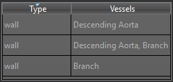
    2. While holding CTRL click the outflow for both outflows of the bifurcation branches (the faces will turn yellow when selected), both the Descending Aorta and Branch should appear in the list below the Properties section

    3. Click the "Select faces" button to finish the surface selection. In the RCR properties tables modify the values of the proximal resistance, capacitance, and distal resistance to match the values listed below

       Property	Value
       Proximal resistance	0.068123
       Capacitance	0.36664
       Disatl resistance	3.1013

       : RCR values for outflows

15. Now all boundary conditions have been specified for the model. Click on the Solver Setup tab and click the "+" button to add a new solver setup. Note solver setup will appear in the Date Manager pane.

    For the properties enter the values as follows

    Property	Value
    CRIMSONSolver solver setup
    Time parameters
    Number of time steps	1100
    Time step size	0.005
    Fluid parameters
    Viscosity	0.004 g/(mm·s)
    Density	0.00106 g/mm³
    Simulation parameters
    Number of time steps between restarts	10
    Residual control	True
    Residual criteria	0.001
    Minimum required iterations	2
    Step construction	10
    Pressure coupling	Implicit
    Influx coefficient	0.5

    : Solver Setup properties

    • The number of times steps × the time step size = the total simulation time, in this case 1110 × 0.005s = 5.5 seconds

    • As the period of the inflow data from the flowfile is 1.1 seconds this results in 5.5 second of simulation time / 1.1 seconds per period = 5 simulation cycles

    • Outputting the restarts every 10 timesteps results in 22 restarts per cycle

    This completes the setup stage.

16. In order to write out files for simulation, CRIMSON needs to know what boundary condition set to associate with the Solver setup.

    1. In the Data Manager pane select the Solver setup and Boundary conditions elements previously created.

    2. Click on Setup Solver

       

    3. Navigate and select a folder (preferably empty) to output the solver files.

17. CRIMSON will output the following files

    • bct.dat

    • geombc.dat.1

    • numstart.dat

    • rcrt.dat

    • restart.0.1

    • solver.inp

    These files will be explained in the following section.