Blood Flow Simulation
In this section the steps required to perform a blood flow simulation are detailed. Using the mesh generated, the CRIMSON Flowsolver solves the 3D Navier-Stokes equations which describe the blood velocities and pressure in our specified geometry.
The CRIMSON Solver has evolved from the academic finite element code PHASTA developed at RPI (Rensselaer Polytechnic Institute, Troy, NY) by Professor Kenneth Jansen. Developed to operate on parallel computer systems, CRIMSON has been used to perform the largest 3D blood flow simulation in the world, operating on 16,384 processors.
Preparing the Simulation
Required Input Files
The input files required for the simulation are generated by the CRIMSON interface. Once again, the following files are generated:
-
bct.dat
-
bct_steady.dat
-
bctFlowWaveform.dat
-
bctFlowWaveform_steady.dat
-
faceinfo.dat
-
geombc.dat.1
-
numstart.dat
-
rcrt.dat (Only generated when using an RCR boundary condition)
-
restart.0.1
-
solver.inp
The contents and purpose of each file listed is given in more detail below.
bct.dat
The bct.dat is the file that contains the information for explicitly imposing the flow data at the inflow face (or at any other face where flow data is imposed).
The bct.dat file contains the nodal values of the prescribed flow rate as detailed in Section 7. The data in this file is stored in text format and can be examined using a text editor. The data in this file specifies the x-, y- and z-velocity components for each node.
bctFlowWaveform.dat
This file contains the inlet flow at each time step of a cardiac cycle for the simulation.
Steady State Files
The _steady.dat version of the bct.dat and bctFlowWaveform.dat files can be used to run a steady state simulation. If you would like to run a steady state simulation, rename the original files to something like bct_pulsatile.dat and bctFlowWaveform_pulsatile.dat and removed the _steady from the steady state files. This is necesarry because Crimson looks for files with the exact names: bct.dat and bctFlowWaveform.dat
geombc.dat.1
The geombc.dat.1 file contains all the geometric information of the mesh, such as the nodal coordinates and connectivity.
faceinfo.dat
This file contains the information for the face on which a boundary condition is applied.
numstart.dat
The numstart.dat file sets the first step number of the simulation, allowing the user to restart the simulation from any previous time step. The data in this file is stored in text format. Here in the bifurcation example we begin at t=0, therefore this value is set to 0. This is generally the case for new simulations.
rcrt.dat
This file is only generated if an RCR boundary condition is being used. The rcrt.dat file contains the parameters of each of the RCR boundary conditions specified in the model.
restart.0.1
Restart files contain information on the pressure and velocity at every point in the mesh.
The restart.0.1 file contains the nodal values of pressure and velocity throughout the model at \(t=0\); restart.1000.1 would represent start from step \(1000\).
solver.inp
The solver.inp file contains the all the instructions for the flowsolver and is built from the solver options set in Section 4.
Preparing files for simulation
Prepare simulation files by clicking on SOLVER SETUP in CRIMSON. This will generate bct.dat, bct_steady.dat, bctFlowWaveform.dat, bctFlowWaveform_steady.dat, faceinfo.dat, geombc.dat.1, numstart.dat, rcrt.dat, restart.0.1, solver.inp and a sub-folder called presolver in the directory you chose.

Modifying presolver files
If you want to modify the any aspect of the initial or boundary conditions without modifying the geometry or mesh, you can re-run the presolver from the command line. The sub-directory generated called presolver has all of the necesarry files to generate a new geombc.dat.1 and restart.0.1 files.
Windows
To run the presolver from the command line, find the path to the presolver in your Crimson installation. It should look something like this:
C:/Program Files/CRIMSON XXXX.XX.XX/bin/Python/lib/site-packages/CRIMSONSolver/SolverStudies/presolver.exe
To make this easier, the executable can be added to the System Path:
-
Press the windows key and search for 'Path'
-
Open the best match option 'Edit the system environment variables'
-
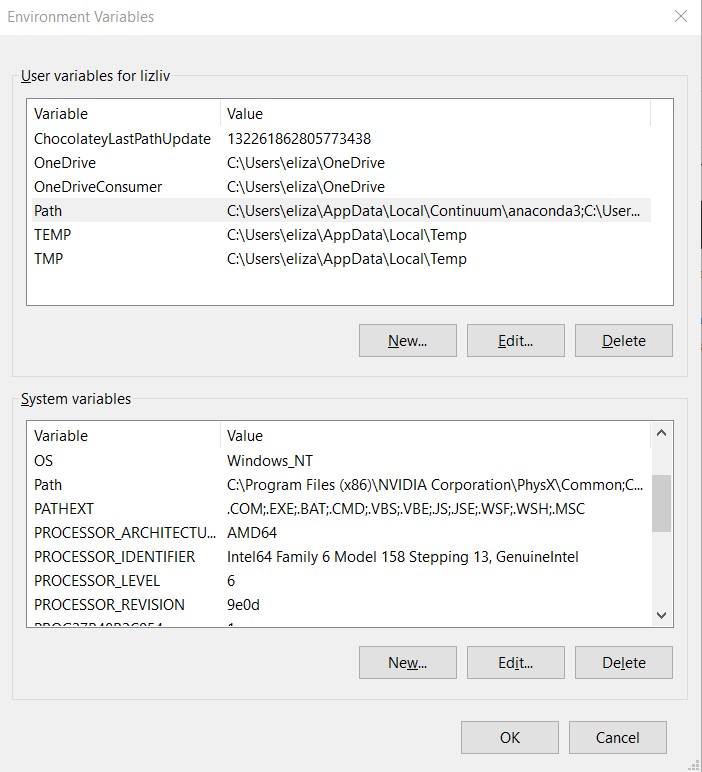
Click the 'Environment variables' button, it will open a new dialogue box
-
The box will have two sections 'User variables' and 'System variables'. In both lists, there is a 'Path' variable with a list of values. If you are the only user on the system, you can add to the 'User' Path, however, if you want this to work on multiple accounts, add to the 'System' Path.
-
Whichever option you choose, select 'Path' in the list and then click the corresponding 'Edit' button. A new 'Edit Environment Variables' dialogue box will open.

- Select 'New' and paste the path to the presolver executable.
Once the presolver is added to the Path, open a new powershell window and navigate to the presolver directory you were modifying. Note: if you already had a window open, you have to close and re-open to load the new system path variables.
The presolver can then be called using the following command:
presolver the.supre
You should see new geombc.dat.1 and restart.0.1 files in the presolver directory.
Preparing Files for Steady/Pulsatile Simulation
-
Copy
bct_steady.dat, bctFlowWaveform_steady.dat, faceinfo.dat, geombc.dat.1, numstart.dat, rcrt.dat, restart.0.1, solver.inpinto a 'Steady' folder, remove the_steadysuffix from the relevant files. -
Copy
bct.dat, bctFlowWaveform.dat, faceinfo.dat, geombc.dat.1, numstart.dat, rcrt.dat, solver.inpinto a 'Pulse' folder -
For Steady Simulation: Transfer the files in the 'Steady' folder into a new folder named 'Steady' on HPC
-
Log into the HPC
-
Navigate to 'Steady' folder and add the following tolerance lines in
solver.inp
vi solver.inp: to open the file and under the linear solver add the followingFor Human Models

For Mouse Models

- Convert the .dat text files to UNIX using
dos2unix *.dat-
Run the simulation
-
Once the Simulation has finished, navigate to the
n-procs-casefolder and transfer PressHist and FlowHist files to your machine -
Examine the PressHist.dat & FlowHist.dat file via MATLAB \(\rightarrow\) check if values converge to a fairly constant value -if this is the case proceed on- if not it maybe be necessary to have more time steps
-
Navigate to the
n-procs-casefolder generated by the simulation you ran-
Combine the parallel files using postsolver
postsolver -sn <stepnumberX> -newsn 0 -ph -td` -
This reduces all the parallel steps till X restarts into a single file
restart.0.0
-
-
Transfer the
restart.0.0into the 'Pulse' folder on your system and renamerestart.0.0asrestart.0.1.
-
-
For Pulsatile Simulation: Transfer the files into a new folder named 'Pulse' on the HPC
-
Follow step 6-7. Once in the solver.inp file edit the Step Construction to 10 iterations as shown below

- Convert the .dat text files from to UNIX using
dos2unix *.dat-
Run the simulation
-
Post-process the results
-
Running Simulations
Now that we have our files prepared, we have a few options for running the CRIMSON flowsolver.
Windows (Local)
One of the simplest ways to run the flowsolver is by pressing the 'Run Simulation' button  in the 'Study' pane of the 'Solver Setup' window:

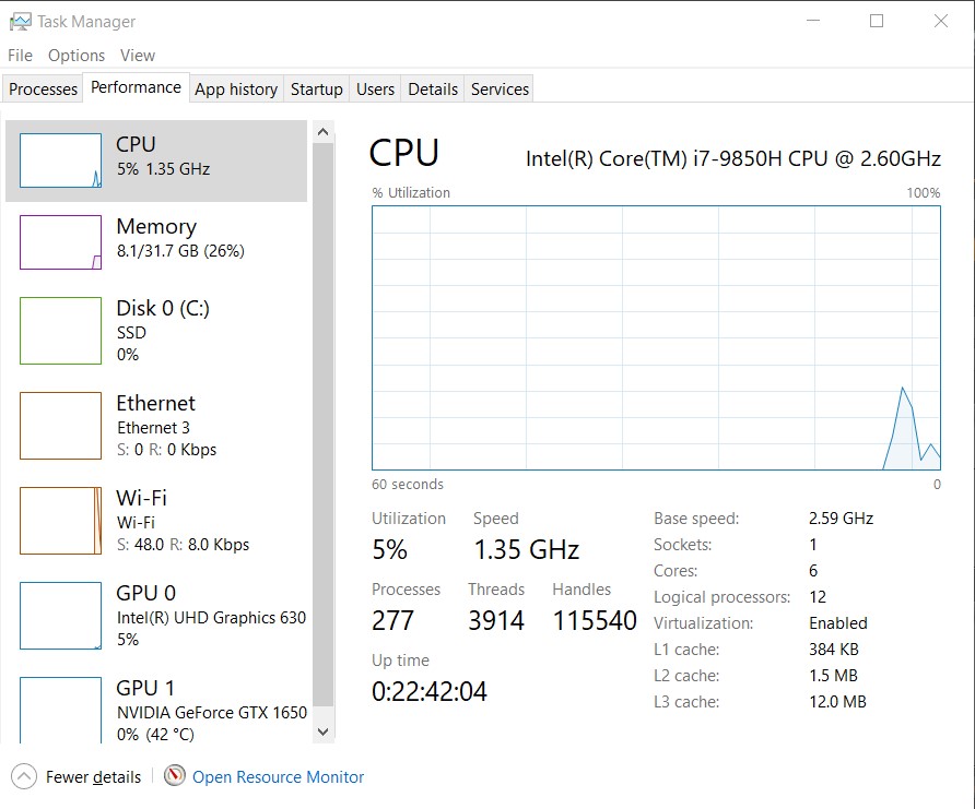
This will open a CMD window with a prompt asking how many processors you would like to use. You can check how many cores are available on your machine by opening the Task Manager, navigating to the 'Performance' tab, and selecting your CPU. The number of cores is the maximum number you can enter for processors in the CMD window prompt.
If you are trying to use your machine for other tasks, you should use fewer cores.

When the solver begins, you will see the output file in the command line:

This file being printed to the command line is histor.dat. It will be discussed in more detail in another section.
The simulation output files will be saved in a new directory called n-procs-case where n is the number of processors for the simulation.

Command Line
If desired, you can also run the flowsolver from the command line.
Following the same path as the presolver, there is another directory for the flowsolver. This has a flowsolver executable, flowsolver.exe and a Windows batch file, mysolver.bat. To run this batch script, navigate to the flowsolver directory in a PowerShell window:
C:/Program Files/CRIMSON XXXX.XX.XX/bin/Python/lib/site-packages/CRIMSONSolver/SolverStudies/flowsolver
You can then run the batch script with the following format:
mysolver <path to simulation folder>`