Boundary Condition Setup

Overview

Boundary conditions are used to represent the pressure and blood flow beyond the boundaries of our segmented model.

To assign boundary conditions, we first generate a "CRIMSON Solver" instance:

Then we can assign boundary conditions within the "Boundary Condition Set":

Boundary Conditions Available

This is the list of boundary conditions currently available in CRIMSON:

• Initial Pressure
• Inlet:
  • Prescribed Velocity (Analytic)
  • Prescribed Velocity (PC-MRI)
• Wall:
  • No Slip
  • Deformable Wall
• Outlet:
  • Zero Pressure
  • Pressure
  • RCR

Basic BC Assignment

For the inlet flow, we can either prescribe a parabolic or plug shaped velocity profile

This is how the velocity is assigned:

For the outlet, we can assign zero pressure, constant pressure, or the physiologically relevant Windkessel model

This is how the Windkessel BC is assigned:

For the walls, we can either have rigid or deformable walls. For rigid wall simulation, we specify a no slip condition:

This is how the no slip is applied:

Initial Pressure

Once we are finished applying boundary conditions, we can set up the parameters of the simulation in the "Solver Parameters" window:

Deformable Wall

In reality arteries are elastic deformable vessels, not rigid structures.

Simulating this requires the coupling of both solid and fluid mechanics.

Blood flow simulation in a thoracic aneurysm model:

To run this type of simulation, we will replace the "No Slip" boundary condition with "Deformable Wall":

Next, we need to assign the material properties to the wall. We will assign a custom rule that defines the thickness of the wall:

Spatially-Varying Material Properties

There are two methods to achieve spatially-varying material thickness:

1. With a table

   Interpolation using a table

   

   Choose the input variable: Position along vessel (d) Local radius (r) Coordinate (x,y,z)

   Input the list of values: Thickness Young’s modulus, Etc…

   – or –

   Load the values from file

2. With a custom script

   Custom Python script

   

   For more complex dependencies Can use all input variables as in previous case Available packages Built-in Python packages Numpy

Finally, you can view the material properties in the model:

PC-MRI Velocity Profile

This feature of CRIMSON allows you to prescribe a 3D (time-dependent) velocity profile at any model inlet or outlet based on Phase Contrast MRI (PC-MRI) data.

This feature is shown through a walkthrough:

The first step is loading in the PC-MRI data alongside the image data used for geometry reconstruction:

As shown above, we create a new boundary condition and assign a "Prescribed Velocity (PC-MRI)" to the inlet face:

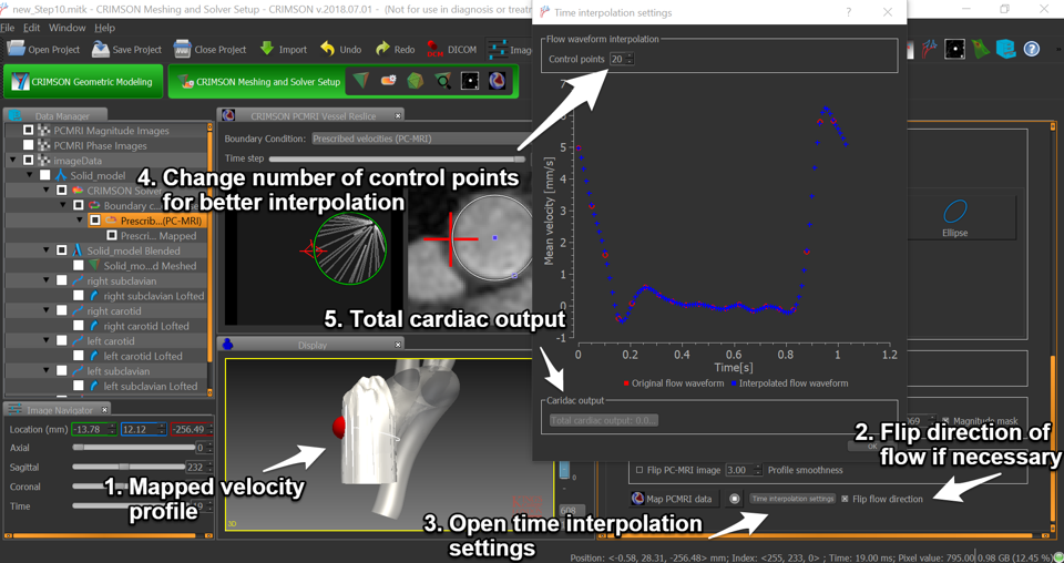
Next, open the PCMRI Vessel Reslice to segment the data, drawing contours for each time step in a cardiac cycle:

Map the data by placing PCMRI and MRA landmarks:

PC-MRI acquisition parameters are necessary to correctly calculate velocities from PC-MRI phase data

The table summarizes the parameters that must be set for each MRI machine manufacturer*:

MRI Machine Manufacturer	PC-MRI format	Velocity encoding (cm/s)	Cardiac frequency (beats/min)	Venscale	Magnitude mask (Yes/No)
GE	DICOM	X	X	X	X
Philips	PAR/REC	X	X

*we currently only possess information about GE and Phillips machines. If you have information about velocity calculations for other manufacturers of MRI machines, feel free to contact us so that we can implement it.

Running the Presolver from CMD line (Windows)

If you want to make small changes to the boundary conditions, you can re-run the presolver from the command line to regenerate the geombc.dat.1 and restart.0.1 files.

The presolver executable can be found in the Crimson installation files, the exact path will depend on the version that is installed and the location. For example:

C:/Program Files/CRIMSON 2020.03.12/bin/Python/lib/site-packages/CRIMSONSolver/SolverStudies

This may be added to the user/system PATH so that the presolver can be run from the command line. Once added, navigate to the presolver directory with the modified files and run:

presolver the.supre

This will generate new geombc.dat.1 and restart.0.1 files in the presolver directory. These files can then be copied along with the other required files to run a simulation.