Scalar Problem Tutorial¶

Files for simulation¶

Important Run/Postprocessing¶

myjob.sh (for submitting the simulation)
mpScalar (for post processing)

Bicarbonate Buffer System (4 scalar simulation in a cylindrical geometry)¶

Oxygen-Hemoglobin Dissociation (3 scalar simulation in a candy cane aorta geometry)¶

Fluid.mitk
Fluid + Scalar.mitk
Matlab Solvers
Reference Paper

I. Setting up the Scalar Simulation¶

Add Scalar Problem Set and Create Scalars¶

Click CRIMSON Solver Setup
Make sure CRIMSON Solver is selected in the Data Manager
Navigate to the ‘Scalar’ tab and create a new Scalar Problem
Add your scalars, then hit okay. You can always add and remove scalars later

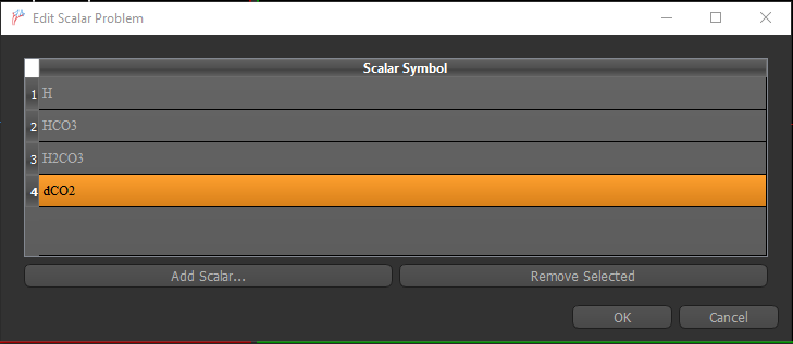
Scalar Symbol and Reaction Constant Naming Requirements¶

All names used in a reaction expression are case sensitive, and must meet all of the following conditions:

Must consist of only the following characters: A-Z, a-z, 0-9 and _,
and, Must not start with a number,
and, Must not be a Python 2.7 keyword

Examples:

III is a valid name, but it will not be treated as the same scalar as iii
“My scalar” is not a valid name, because it contains a space (‘ ‘)
“My_scalar” would be a valid name
“2Scalar” is not a valid name, because it starts with a number
“Scalar#3” is not a valid name, because it contains the character ‘#’
“or” is not a valid name, because it is a python 2.7 keyword

Note: Changing Scalar Symbols If later on during your work, you need to change the symbol of a scalar, do not double click on the node to rename it. This will only rename the node itself, but it won’t change the scalar’s symbol.

Instead, use the “Change scalar symbol” button in the scalar tab.
As of the time of writing, Crimson does not adjust your reactions or iterations to accommodate the new scalar name. You will need to manually adjust these if you rename a scalar.

Scalar Node Parameters¶

Diffusion Coefficient¶

The diffusion coefficient is the value D in the Reaction-Advection-Diffusion equations that describes how quickly a species will be transported via diffusion through the fluid.

Residual Control / Residual Criteria¶

This feature is not implemented in the scalar flowsolver yet and does not work, but it will be implemented in the future. Do not use.

Currently the flowsolver will disregard what value you enter into this field, future versions of the flowsolver may make use of it to stop simulation automatically when the residuals go below the residual criteria that you set.

Add Reaction Coefficients¶

Select Scalar problem set in the Data Manager
Select Edit Reaction Coefficients
Add your Reaction Coefficients

Edit Reactions Terms¶

Repeat this process for all scalars
Select your scalar in the data manager
Click Edit Reaction
Enter your Scalar Reaction then hit ‘Test Reaction’. Remember that the reaction you are entering is how the scalar changes with respect to time.
Successful Reaction
Add a reaction to each scalar
Save after this step

H dy(1)= k2H2CO3 - k1H*HCO3;

HCO3 dy(2)= k2H2CO3 - k1H*HCO3;

H2CO3 dy(3)= k1HHCO3 + k4dCO2 - (k2 + k3)H2CO3;

dCO2 dy(4) = k3H2CO3 - k4dCO2;

1-D MATLAB solver to test your reactions - Driver - Reactions

Reaction Equations¶

The ^ symbol does not mean “to the power of”
The ‘ symbol does not mean “transpose”, avoid using this symbol
Use for “to the power of”, for example, II3 means “scalar II to the power of 3”
Reaction expression strings must be valid Python expressions
Be careful about accidental use of , k1*I is very different from k1I
The intended use is to type polynomial expressions for reaction equations, e.g., k1II 3III 4 + k2*IV 2
The “Test run” button can be used to check for typos
Check the mbilog console for extra information relating to your reaction
Newlines in the reaction equation are only for display purposes, all newlines will be stripped * before the expression is written to scalarProblemSpecification.py and executed
It is not necessary to specify the left hand side gradient of a reaction expression, there is code to generate this expression automatically

Things to avoid¶

Under no circumstance should you add # comments anywhere in your reaction expression, since newlines are removed, you could easily accidentally comment out most of your reaction
In theory string comments like ‘this is a comment’ may be OK, but it’s not recommended.

Unsupported operations¶

The reaction expression is executed as Python code, but the following operations are not recommended (and may cause unexpected results): * Using the equals sign (=) anywhere in the reaction * Function definitions * Lambdas * Conditional logic * Boolean expressions * Strings (you might accidentally make your whole equation a string) * Accessing other Python classes in PythonModules * Writing to a file / doing other operations that have side effects that are retained between iterations.

If you need to do any of these things, I recommend just making your own version of scalarProblemSpecification.py and making your edits there, contact the mailing list if you need help.

Peclet Number¶

It is good practice to calculate the peclet number for each of your scalars

The Pé number is defined as:

\[Pe = \frac{\textrm{advective transport rate}}{\textrm{diffusive transport rate}}\]

For mass transfer, it is defined as:

\[Pe_L = \frac{Lu}{D}=Re_L Sc\]

where \(L\) is the characteristic length, \(u\) is the local flow velocity, and \(D\) is the mass diffusion coefficient.

  L = 13.78 mm (pipe diameter)

  mew= flow rate/Area

  Flow rate= 33,333 mm3/sec

  (from prescribed velocities inlet condition)

  area= 596.608 mm2

  (from contour information)

   mew= 55.87 mm/s

  D = 1.1 mm^2/s

  (automatically set in each scalar’s tab)

  Pe = 700

A high peclet number means that our scalar simulation is much more dependent on advective flow rather than diffusive flow => the flow field is responsible for the scalar’s motion

Edit Scalar Boundary Conditions¶

Repeat this step for all scalars
Select your scalar in the Data Manager
Click Add or Edit Boundary Conditions
Add the following boundary conditions: No Flux, Consistent Flux, Initial Concentration, and Scalar Dirichlet
Boundary Condition Parameters

a. No Flux
- Hit Apply to all walls
b. Consistent Flux
- Select the cylinder outflow
c. Initial Concentration
- Leave at 0 mmol/L
d. Scalar Dirichlet
- Select the inflow and add the specific inflow value you want for your scalars
Add boundary conditions to each scalar
Save after this step

Scalar Boundary Condition Types¶

No Flux¶

The “No Flux boundary condition is equivalent to prescribing a zero-Diffusive flux boundary condition. In the case of a rigid-wall simulation, the “No Flux” condition acts as a zero-total flux boundary condition due to the zero velocity at the walls. The application of the “No Flux” condition on all walls prevents scalar concentration from “leaking” through the walls during a simulation. In the case of an FSI simulation where the velocity at the walls is not equal to zero special consideration should be taken.

Initial Concentration¶

The initial concentration sets the scalar concentration of your entire domain at time t = 0 to a specific value. Users specify a separate initial concentration for each scalar species.

Neumann¶

The Neumann boundary condition specifies the derivative (slope) of the scalar species perpendicular to the boundary face. This corresponds to the flux of scalar concentration across a boundary.

Dirichlet¶

The Dirichlet boundary condition sets the scalar concentration to a given value at a boundary face for all points in time.

Consistent Flux¶

The Consistent Flux boundary condition is a type of Neumann boundary condition that iteratively specifies the diffusive flux of the given scalar species at an outlet face based on the most recent scalar solution. The Consistent Flux outperforms the standard Zero-Diffusive boundary condition in terms of accuracy for low Péclet number problems and yields the same solution at higher Péclet numbers. We recommend using this boundary condition for outlet faces. Details can be found in DOI: 10.1002/cnm.3378.

Edit Scalar Solver Parameters¶

Select the Solver parameters 3D tab in the Data Manager
Click Edit Solver Iterations
Add Solver Iterations for each scalar. Scalar symbols are case sensitive For more in-depth editing you can copy/paste from a spreadsheet program like Microsoft Excel
Hit OK and return back to the solver parameters
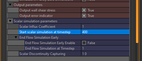
Change Start scalar simulation at timestep to 400. This allows the flow field to stabilize before running the scalar simulation
You are almost ready to start your first scalar simulation!

Scalar Parameters¶

Scalar Influx Coefficient¶

This influx coefficient enables solving numerically stable scalar problems under conditions of transient flow. This formulation is analogous to the Influx Coefficient for the flow problem. We recommend keeping this value set to 1.0. Details can be found in DOI: 10.1002/cnm.3378.

Start Scalar Simulation at Timestep¶

Set this to a value other than timestep 1 if you would like to run a few timesteps with only the fluid solver as part of your simulation
You may want to do this if you want to let the fluids “settle out”
Timesteps are 1 based.
Note that a timestep is not an iteration number. Each timestep consists of a set of fluid iterations and scalar iterations.

Example 1

  Settings:
  Start Scalar Simulation at Timestep = 10, 
  End Flow Simulation Early: Disabled

  Result:

  Timesteps 1 through 10: Only fluid iterations will be ran.
  Timesteps 11+: Fluid and scalar iterations will be ran
  End Flow Simulation Early

If you want to stop running the fluid iterations after a certain number of timesteps, but continue running the scalar iterations after that time, enable this option and set “End Flow Simulation at Timestep” to the timestep that you want to stop doing fluid iterations on.

Example 2

  Settings:
  Start Scalar Simulation Timestep = 10
  End Flow Simulation Early: Enabled
  End Flow Simulation at Timestep = 100

  Result:

  Timesteps 1 through 10: Only fluid iterations will be ran
  Timesteps 11 through 100: Fluid and scalar iterations will be ran
  Timesteps 101+: Only scalar iterations will be ran

Scalar Discontinuity Capturing (DC)¶

This is an additional form of stabilization for the scalar problem that helps resolve the issue of spurious oscillations in the solution at wavefronts for high Péclet number problems. Using the scalar DC stabilization makes the transport equations nonlinear and adds a small increase to the computational cost of simulations. Details can be found in DOI: 10.1002/cnm.3378.

If this option is checked in Solver Parameters, this stabilization will be enabled.

Scalar Iterations¶

About the Solver Iteration Sequence In a scalar simulation, for each timestep of the simulation, the flowsolver follows this process:

Timestep 1

Fluid iterations
Scalar iterations

Timestep 2

Fluid iterations
Scalar iterations

... (repeat for N timesteps)

The fluid iterations always run before the scalar iterations on a given timestep

The scalar iterations are of the form:

Scalar < some scalar > for < some amount > of iterations
Scalar < some scalar > for < some amount > of iterations
Scalar < some scalar > for < some amount > of iterations …

Example scalar iterations for a timestep:

Scalar III for 5 iterations
Scalar II for 3 iterations
Scalar V for 8 iterations
Scalar II (again) for 8 iterations
Scalar III (again) for 2 iterations

The scalar iterations can happen in any order, and the same scalar can be repeated multiple times in a given timestep.

II. Create Simulation Files¶

Configure Solver Study 3D¶

Click CRIMSON Solver Setup
Select Solver study 3D in the Data Manager
Enable Scalar Problem set and select your Fluid Boundary Conditions
Click Setup Solver and then choose a suitable location for your simulation files. Be patient with CRIMSON, the mbilog will tell you when solver setup has finished