 GEOGRAPHY:
SPATIAL ANALYSIS, THEORY AND PRACTICE
NRE530 (3 credits)
SCHOOL OF NATURAL
RESOURCES AND ENVIRONMENT
THE UNIVERSITY OF MICHIGAN

Class Resource Page
Professor Sandra Arlinghaus (Ph.D.)
Wednesdays, 6-9 p.m.
Dana Building 2046 (class)
Office in Dana: 2044
Research office: 1130 Hill Street (Community Systems Foundation:
CSF)
Phone: 761-1358 (research office); 975-0246 (home, between 9 a.m. and
9 p.m.)
e-mail: sarhaus@umich.edu (preferred method of communication)
Office Hours: Monday (CSF), 10a.m. to 3p.m.; Wednesday(Dana), by appointment
after class (and possibly before class); Thursday (CSFor Dana; call CSF
(761-1358)), 10a.m. to 3p.m.; and, by appointment.
COURSE DESCRIPTION
A spatial view of the environment is one that often
involves maps. As the context in which one views an environmental
issue is a critical matter, so too is the context in which one views a
map. Thus, the exciting state-of-the-art electronic mapping capability
of Geographic Information Systems (GIS), and of other mapping software,
is cast in the broader context of geography and mathematics--the theoretical
foundations from which GIS is derived.
Isolationist views, from the environmental to the
political, cannot survive in the world of the geographically literate.
Creative, scientific approaches to topics, using well-established but untapped
tools are envoruaged, as are traditional approaches which clearly exhibit
the spatial components of an environmental problem with suggested directions
for action. Students learn mapping in the context of project development.
In careful collaboration with the instructor, each student builds a document
and presentation to enhance his/her research and teaching portfolio.
All software used is for the PC.
University computing sites should have ArcView GIS available.
All software used in the course will be available for use on a machine
in 2044 Dana.
COURSE MATERIALS
-
Web page and attached materials
-
Electronic resources of various sorts: lectures, links to articles,
and so forth
-
Holdings of the map library
-
Each student is required to have an active e-mail account; e-mail will
be a critical tool
-
Each student should set up a web page, early in the course. The
web will be used for on-going communication between student and instructor
and with student colleagues.
COURSE RESOURCES, AFTER THE FACT
Student work will be displayed on bulletin
boards, both actual and virtual, as appropriate. Some individuals worked
together in groups; grouping has been retained here and is denoted by cell-background
color coding. Individuals presenting material alone have cells of
background color white.
VIRTUAL BULLETIN BOARD: CLICK ON LINKS TO SEE PROJECTS
Rosalyn Scaff
City of Ann Arbor, Neighborhood and Commercial Associations |
Da-Mi Maeng
Maximum Projected Land Development: An Analysis
of Full Build-out Development, Pittsfield Township, Washtenaw County,
MI |
Suzy Brunzell
Landsat TM Band Combinations |
Ray Stemitz
Can I Live on Mars? A Middle School Exploration
of our Solar System |
Renee
Rosingana
Detroit Elementary Schools Located in Area B |
Danielle Dipert
UM Residence Hall and Family Housing Maps |
Erez
Bar-Nur
Mallett's Creekshed |
Mark Elwell
The Remote Sensing of Volcanic Ash Cloud |
Bebe Lloyd
Binomial Theorem and Map Coloring: Snow White and
the Seven Pixels |
Millicent
Fisher
Detroit Elementary Schools Located in Area B |
Thana Chirapiwat
Analysis of Energy Consumption of the University of Michigan's
Buildings |
Karen
Lawrence
Mallett's Creekshed |
Ken MacLean
Mapping Ethno-linguistic diversity in N. Vietnam |
John Ley
The Students' Cell Page |
Brian
Toth
Detroit Elementary Schools Located in Area B |
Joe Holtrop
Michigan Conservation Districts and Farmland Protection
Journal
Mapping Appendix: 1,
2,
3,
4,
5,
6,
7,
8,
9,
10,
11,
12,
13,
14,
15,
16,
17,
18,
19,
20,
21,
22,
23
Final Maps: 1, 2 |
Myloc Nguyen
Huachuca Mountains |
Stephanie
Motyka
Spatial Analysis of Chemical Bonds |
Mary Ann
Villar
The United States of America: A Journey through
Time |
Kevin
Collins
Detroit Elementary Schools Located in Area B |
Erik Wetzler
Backpacking Michigan's National Forests |
Elizabeth
Worzalla
Huachuca Mountains |
Jennifer Rifkin
Spatial Analysis of Chemical Bonds |
Matt Austin
The United States of America: A Journey through
Time |
William Thompson |
Qiang
Hong
Travel Patterns and Social Demographic Characters of
SMART's Riders in Three Counties of Metropolitan Detroit |
Jen Abdella
The AuSable River: a preliminary spatial analysis
of landscape and instream characteristics which may affect distribution
of brown trout
(Salmo trutta) and walleye (Stizostedion vitreum) |
Amy McCullouch
Astronomy for Kids:
Mapping the Stars |
Gabrielle
Burba
U.S. History Resource Page |
Lily Le
Whitney
Promoting Positive Youth Development with Education-
and Community-Based Nonprofits in Washtenaw County |
Tamar Noam Glazer
Travel Patterns and Social Demographic Characters of
SMART's Riders in Three Counties of Metropolitan Detroit |
Steven Perrine
Freshwater fish distribution as a function of relative
body depth and river gradient. |
Anna Mosher
Astronomy for Kids:
Mapping the Stars |
George
Darden IV
U.S. History Resource Page |
Steve Eschrich
Promoting Positive Youth Development with Education-
and Community-Based Nonprofits in Washtenaw County |
FORMAT
Casual lecture and discussion (your participation
is vital); a research format. Student success in this sort of research-style
format depends heavily on students working on a regular and continuing
basis throughout the term.
EVALUATION:
-
Middle of term: Hand in draft of project as mid-term and give formal 5-7
minute (depending on class size) oral presentation: 25% of grade.
-
Two weeks before end of term: Presentation of most of final project as
a talk (formal 5-7 minute oral presentation, depending on class size):
25% of grade.
-
Day of scheduled final, Final project (website or other) is due by 5 p.m.:
Final project--: 50% of grade.
The formal oral presentations are designed to give students experience
in a friendly setting of the kinds of constraints they will meet when presenting
papers at professional meetings. The final project may be a term
paper, a chapter in a thesis, a substantial website, or other selected
in consultation with the instructor. Hard copy should be prepared
using Microsoft Word for Windows using 1 inch margins on all sides, 12
point type, double-spaced. Notes should be gathered as endnotes.
Graphics may be cut into Word from a variety of packages. Instructor
is quite willing to help individuals needing it with help in word processor
use or website development.
Students will have the opportunity each time to discuss matters of concern
and to get feedback on a regular basis as needed.
LECTURE MATERIALS--TENTATIVE SCHEDULE; MAY ALTER TO SUIT NEEDS.
LECTURE 1
-
Sign-up sheet with names, ssn, and e-mail addresses
-
Create Wait List if needed.
-
Presentation of course web page (this page)
-
Brief introductions
-
Brief written ideas of interests of each student
Practice
-
Mapping: brief demonstration
Theory
Practice
-
Creation of simple web page
-
Assignment 1:
Get e-mail account
Get familiar with the course home page
Look around on the web
Make simple home page
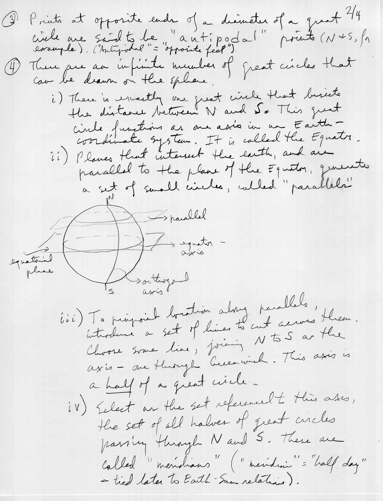
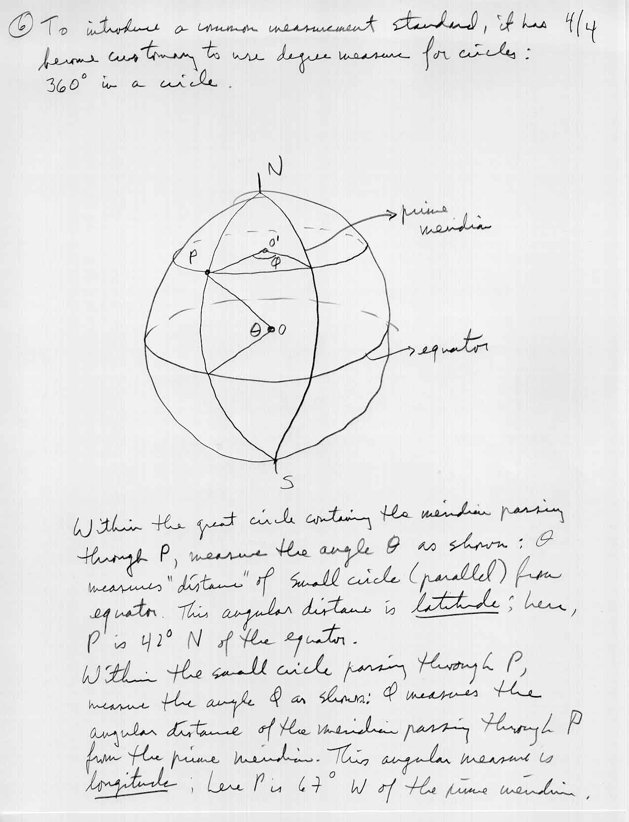
Review latitude and longitude material covered in class
Get comfortable using ArcView to make a simple thematic map
LECTURE 2
Theory
Practice
-
Maps
Animal Movement and Spatial Tools, USGS extensions requiring Spatial
Analyst Extension to ArcView 3.0a--one sample: Ann
Arbor Parks another sample: triangulated
irregular network
U.S. by County--thematic maps
Wayne County--by census tracts
LECTURE 3
Practice
-
PhotoShop demonstration using maps
-
Multiple layers on maps
LECTURE 4
Theory
-
Challenge: find a map on the torus requiring seven colors.
Practice
-
Sample project creation
-
Base map opened in ArcView
-
Data brought in and linked to map; open up the attribute table that
goes with the map. Then add a new table (.dbf file--can be your own,
made in Excel and saved as a .dbf). On the added table, click on
the column heading containing the two letter country code (for example);
on the attribute table, click on the corresponding column heading.
Click on the "join" button at the top. Now the added data can be
used to make thematic maps. Material concerning
"joining" and "linking" tables to maps in ArcView.
-
Thematic map created
-
Map exported to PhotoShop
-
Map saved in .gif format
-
Use of MapEdit to make map clickable; works for any .gif--so, any map
from any GIS or any photo or scanned image saved as a .gif.
In MapEdit, make sure neither "radio button" is checked on launching
the software
In putting in URLs for hot spots, test the URLs and reinsert unusual
symbols, such as tildes and dashes that do not "stick" the first time;
they will stick the second time.
Save the file as .htm, a client-side file.
-
Upload the file to the web. Check that in fact it works.
-
MapEdit is shareware: http://www.bhs.com
-
DEMs (Digital Elevation Models)--another source for base maps or backdrops.
-
Find USGS site (www.usgs.gov) and source for DEMs (http://edcwww.cr.usgs.gov/nsdi/gendem.htm)
-
Download from 1:250,000 (1 degree) series; choose the "by state" category,
for example. Navigate to save the file to your local computer.
-
Once the file is downloaded, run WinZip on it (download that from www.shareware.com)
or unzip in some other way. The file is in the .gz format.
In WinZip, you will need to run "classic" mode when prompted, click on
the file name, and then "extract".
-
Then, you will be able to open the DEM in ArcView with Spatial Analyst
loaded. Choose File|Import Data Source, and then pull down the menu
to choose USGS DEM.
-
You might then want, under "theme," to choose to convert this file to
a shapefile ("convert to shapefile").
-
Possible resource: older curve-fitting files. 1.
2.
3.
4.
5.
6.
7.
8.
-
Possible resource: article
on downloading Digital Line Graphs from USGS site.
LECTURE 5
Theory
Practice
-
GIS links base map and data set in an interactive manner.
-
Base maps: last time we used a map from ArcView as a base map
for making a clickable webmap; there are numerous other sources of base
maps.
-
Street Atlas 4.0, base maps. Copy map to clipboard and paste into
PhotoShop. Save as a .gif and as a .jpg.
-
Use the .gif in MapEdit as the base for a clickable map.
-
Use the .jpg in Atlas GIS as a background for a GIS map; insert symbols
as needed to reflect, say, street locations. Then use as a base map,
for a clickable or other map.
-
Digital Chart of the World: vectorized format to bring in to work
seamlessly in Atlas GIS. Use to make base map. DCW contains
files of things that can be seen from the air--for the entire world.
Contains topographic contours, 1000 foot contour interval.
-
Maps on the web: USGS last time. University
of Texas at Austin, Perry-Castaneda collection of maps are useful political
maps. These also can be used as backdrop in a GIS.
-
Global data source: World Resources Institute Database.
-
Animated maps; Movie Gear. Animate final maps: animated
maps can be effective in showing change over time. See "animaps"
for some samples.
General suggestion: often it is helpful to begin a big project
by breaking off a piece of it as a "pilot" project. Use the pilot
project to nail down your strategy, debug your methodology, and fine tune
your analysis. Then when it comes time to extend to a broader context
you will be pretty well set to do so!
LECTURE 6
Theory
Practice
-
Earlier we brought new data into the GIS and linked it to the map.
Also, we identified other sources of existing images. Now consider
creating your own image. No matter how you do it, you need to consider
whether or not the image you are creating will fit into an existing map
(if you care about this issue). That is, you need to know that the
PROJECTION of the map you are creating will fit into (for example) a map
of the State of Michigan.
-
One way to bring in an image is to scan it. A scanned image itself
is not directly useful in a GIS, although it may well be useful as a background
image. To make it useful, it is necessary to convert its format from
"raster" to "vector."
-
One way to achieve this conversion is to electronically "trace" the
map into the GIS: a process called digitizing. There are a
number of ways to digitize an image.
-
One way to digitize is to use a digitizer (a special piece of equipment);
another is to do onscreen digitizing.
-
One way to do onscreen digitizing is to open up Atlas GIS and use the
capability present there--demonstration follows. (Or use ArcView
with Spatial Analyst Extension).
-
Once both images and data sets are in place, there are a number of analytic
tools that are available in the computing environment. To date, we
have been looking at conceptual, analytic tools that underlie the broad
base of the entire mapping environment. These are critical to understand
(consider what happened when the Jordan Curve Theorem was not accounted
for !!).
-
There are also more local analytic tools that are often useful in crafting
individual maps. One is called a "buffer"--for example--demonstration
follows:
-
a buffer might be a circular region surrounding a school--one could
count the number of people that fall into that buffer if one were considering
distances students need to walk to school.
-
Or, one could buffer a line segment and count the number of census block
groups that intersect this "sausage".
-
Or, one could create a sequence of concentric circles as buffers of
varying distance.
-
Or, one could create a sequence of concentric rings as buffers of varying
distance.
LECTURE 7
Theory
Practice
-
Three-dimensional maps.
-
Resource: conversion file directions
-
Trouble-shooting and matters related to presentations.
LECTURE 8--GIVEN BY STUDENTS IN CLASS, 18 PRESENTATIONS, 5-7 MINUTES
EACH, NEW PRESENTATION EVERY 10 MINUTES (I WILL BRING A TIMER). PLEASE
KEEP YOUR PRESENTATION TO WITHIN THE LIMIT. PRACTICE IT, WITH A TIMER,
AHEAD OF TIME. LEAVE TIME FOR SOME FEEDBACK FROM THE CLASS.
LIST OF PRESENTATIONS:
Local (state or larger scale studies)
Rosalyn Scaff -- poster maps
and web presentation
Danielle Dipert -- web presentation
Thana Chirapiwat -- web presentation
Joe Holtrop -- overhead presentation
Erik Wetzler -- web presentation
Qiang Hong and Tamar
Noam Glazer -- web presentation
Da-Mi Maeng -- PowerPoint presentation
Erez Bar-Nur and Karen
Lawrence -- poster maps, overhead, and slide projector presentation.
Regional
Myloc Nguyen and Elizabeth
Worzalla -- poster maps and web presentation
Jennifer Abdella -- web presentation
Stephen Perrine -- overhead presentation,
pin map, and web presentation
International
Suzanne Brunzell -- poster maps,
PowerPoint, and web presentation
Mark Elwell -- web presentation
Kenneth MacLean -- web presentation
LECTURE 9--GIVEN BY STUDENTS IN CLASS, 18 PRESENTATIONS, 5-7 MINUTES
EACH, NEW PRESENTATION EVERY 10 MINUTES (I WILL BRING A TIMER). PLEASE
KEEP YOUR PRESENTATION TO WITHIN THE LIMIT. PRACTICE IT, WITH A TIMER,
AHEAD OF TIME. LEAVE TIME FOR SOME FEEDBACK FROM THE CLASS.
LIST OF PRESENTATIONS:
Chemistry application
Stephanie Motyka and Jennifer
Rifkin -- web presentation
Astronomy application
Raymond Stemitz -- web presentation
Amy McCullouch and Anna
Mosher -- web presentation
Mathematics application
Beatrice Lloyd -- web presentation
Biology
John Ley -- web presentation
History application
Matthew Austin and Mary
Ann Villar -- web presentation
Gabrielle Burba and George
Darden IV -- web presentation
Local Michigan
Kevin Collins, Millicent
Fisher, Renne Rosingana, and
Brian
Toth -- web presentation
William Thompson -- web presentation
Steven Eschrich and Lily
Le Whitney --
LECTURE
10 --the process of project development
Theory and Practice
-
Large datasets, that are standardized (held to some known standard),
offer an interesting set of issues (illustrated using Joe Holtrop's work):
-
Obtaining data from the web and saving it as an Excel spreadsheet
-
Highlight the data and go to Edit|Copy in Netscape
-
Then, open up Excel and go to Edit|Paste--this pastes a text copy of
the website information into Excel.
-
To make the text in Excel convert to a spreadsheet, go to the Data pulldown,
choose "text to columns" and choose "fixed width"--now the spreadsheet
can be manipulated easily.
-
Making a master spreadsheet from multiple downloaded smaller spreadsheets.
-
Open up a new spreadsheet and enter the names of geographic units in
the first column (counties in Michigan, for example).
-
Then, highlight columns of data corresponding to each county--note,
that you will need to convert this to row (as opposed to column) data.
Use the Control key to highlight disjoint sets of data. Now, go to
Edit|Copy.
-
Go to the master spreadsheet. Click on the left hand end of the
row into which you wish to paste the data. Pull down Edit|Paste Special
and choose "Transpose" and hit OK. Now the columnar data has become
row data: a column vector had the matrix transpose operator applied
to it to make it a row vector.
-
Repeat the process as needed to make a complete spreadsheet.
-
Save the spreadsheet as a .dbf file and it is an easy matter to link
it up to existing boundary files in a GIS (ArcView used here) available
from various sources (such as the Census).
-
Small datasets and those that are not standardized exhibit a different
set of issues (illustrated using Tamar Noam Glazer and Qiang Hong's work):
-
Data was obtained from field work
-
define spatial regions using "spider diagrams"--origin/destination data
offers insight into spatial linkage patterns and these offer "spot elevations"
around which to contour--each spider lies wholly within a region.
-
bring in established data sets and boundary files to overlay on the
newly-regionalized map.
-
query the data base to create buffers of various sorts as a way to group
data in relation to the regions and distinguished points/lines in them.
-
consider using dot density maps to look for pattern within the spider-generated
units. Scale transformation is critical with dot density maps.
-
if the data is randomized at the block group level, then the pattern
of clustering of dots is meaningless at that scale.
-
shift to a smaller scale map, such as a tract map, to assign meaning
to the pattern of clustering.
-
choice of randomization level depends on the eventual view one wishes
to have: randomizing at the block group level might not make sense
if what one wished were a national view (the dots would all blend together).
However, always choose a randomization level of larger scale that the "view"
scale.
LECTURE 11
Theory
-
Spatial Autocorrelation. How are regions clustered in space?
Are similar ones next to each other or are dissimilar ones next to each
other.
On
this map, all non-white Block Groups whose adjacent Block Groups are
also only non-white are light green.
All non-white Block Groups adjacent to white Block Groups are darker
green
All white Block Groups adjacent to non-white Block Groups are darker
purple.
All white Block Groups adjacent to only white Block Groups are light
purple.
This
map shows a pattern similar to the first one, but with adjacency counted
through two stages.
In both maps, when Block
Group boundaries are removed, a continuous pattern
emerges.
Policy makers and municipal
authorities may find maps such as these useful.
Practice
One procedure for making such maps involves using the query tool
(in Atlas, for this example.
To pick out all block groups in which Nonwhite population dominates
(layer test)
Query|Select by Layer
: choose the blockgroup layer
Query|Select by Value:
choose blockgroups; select subset, by expression,
nonwhite-white>0
Edit|Copy to Layer, Selected
features only, copy features to new layer--region, called "test"
To pick out all block groups in which White population dominates
(layer test2)
Query|Select by Layer
: choose the blockgroup layer
Query|Select by Value:
choose blockgroups; select subset, by expression,
nonwhite-white<0
Edit|Copy to Layer, Selected
features only, copy features to new layer--region, called "test2"
To pick out all block groups that are touching a dissimilar blockgroup:
use test and test 2.
Query|Select by Location|Touching:
then, use test followed by test2 to select nonwhite block groups touching
white block groups.
Query|Select by Location|Touching:
then, use test2 followed by test to select white block groups touching
nonwhite block groups.
Note the lack of symmetry
in adjacency once content is assigned to the blockgroups even though strict
adjacency is symmetric (if A is adjacent to B then B is adjacent to A).
Theory
LECTURE 12
Theory
-
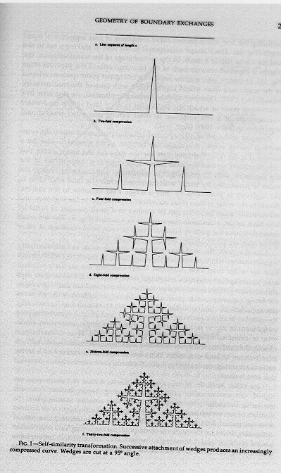
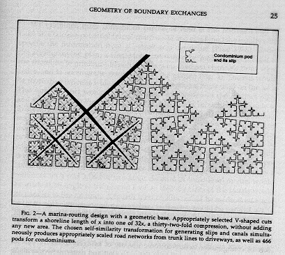
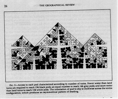
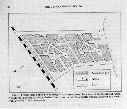
Fractal geometry and minimax principles; human use of environment.
Reprint of selected material from article from the Geographical Review,
published by the American Geographical Society; January, 1990. Article
appears on pages 21-31 of that journal. Selected material:page
1; page 2; page 3;
page
4; page 5.
Practice
-
Map Appreciation--classical cartographical tools--hands-on display
-
Web strategy
-
If you link to another site, inform that site by e-mail and offer to
disconnect if your site becomes a high volume site...at their request.
-
Grabbing an image
-
request permission to use and behave according to answer to request;
-
give cutoff date;
-
put in own directory to avoid bandwidth drain
-
cite source
-
Do not use an image if there are disclaimers on it;
-
U.S. Government materials; these do not generally require written requests
for printed materials...so, apparently, use them...cite source and so forth
and send a request if it indicates that one should be sent.
-
Link to search engines...do not inform them. Cite them:
"here's what Yahoo says about Leelanau...", copy link and paste...pass
along your search skills...can increase traffic on your site.
-
Enter course web page and individual web pages separately in search
engines.
-
Assemble on 530 web page and list that in search engine.
-
Student UM accounts can be kept past graduation (contact Alumni Association)
-
Outside US copyright and related laws/ethics vary.
-
Citations...be clear about where in the documents references are used.
-
Concepts...tie to concepts...those listed above as well as a host of
other: centrality, hierarchy, density, to name a few.
-
Trouble-shooting session
DECEMBER 9, 1998
Student final presentations. Order that appears
as of Sunday, December 6, 11:59 p.m. is the final order.
Presentations related to mathematics and physical sciences:
jrifkin and smotyka
bblloyd
akmosher and almc
rstemitz
Presentation related to social science, history, and planning:
gburba and gwdiv
lilypad and eschrich
qhong and tamarng
dmaeng
DECEMBER 16, 1998
Student final presentations. All final projects are
due.
Presentations related to biological sciences:
jaley
eworzall and mnguyen
jholtrop
jena
smp
Presentations with an international character:
maclean
moelwell
suzyb
Presentations related to social science, history, and planning:
erikwetz
mvillar and mcaustin
kcollins, btoth, fisherma,
and rarosing
erezbzzz and kjlawren
rosscaff
tnac
dkdipert
PARTY AFTER THE LAST PRESENTATION AT
SANDY'S HOUSE, DECEMBER 16.
GIS PACKAGES AVAILABLE FOR USE:
-
Atlas GIS, ESRI
-
ArcView GIS, ESRI
-
MapInfo GIS
-
Excel in Office 97
MAPPING PACKAGES AVAILABLE FOR USE:
-
DeLorme Street Atlas and related packages
-
CelAssembler for making animated maps
-
MapEdit for making clickable maps
-
Visual Explorer from WoolleySoft for making 3D maps
OTHER PACKAGES OF PARTICULAR VALUE:
-
Microsoft Word
-
Microsoft Excel
-
Adobe Photoshop
-
Microsoft Power Point
LABORATORY TOPICS SELECTED FROM AMONG THE FOLLOWING AND IN RESPONSE
TO STUDENT NEED
Reductionist approach:
-
Use of a GIS using on-board data and maps
-
Use of a GIS using imported data with on-board maps
-
Use of a GIS using imported (or on-board) data with imported maps
Routine skills:
-
Strategies for saving files
-
Use of real-world databases and spreadsheets
-
Use of Photoshop
-
Use of PowerPoint
Mechanics of mapping:
-
Single variable thematic maps
-
Choosing reasonable ranges for mapping themes
-
Default color selection and alteration of the default
-
Two variable thematic maps
-
Layers and problems in handling multiple layers
-
Inverse and direct relationships displayed cartographically
-
Alternate coloring; problems associated with making black and white maps
-
Analysis using buffers
-
Maps in PhotoShop
-
Animated maps
-
Clickable maps
-
3D maps