|
ME
574 PROJECT |
 |
||||
|
An
Axisymmetric
Model for Pore-Grain Boundary Separation |
|||||
|
|
|||||
|
|
|||||
During the process of updating the nodal positions by the explicit Euler method or fourth-order Runge-Kutta method, some elements shorten and others elongate. There are two drawbacks: 1. A very short element reduces the time step leading to a very long simulation. 2. A very long element does not capture the curved geometry well. Thus, we include a Matlab function to control the length of the elements. In this function, we prescribe a minimum and maximum element length. If during the evolution of the grain boundary and pore, the element becomes shorter than the prescribed value, it will be eliminated. On the other hand, if it gets longer than the prescribed value, it will be broken in two elements. Another problem that was encountered during the implementation of this finite element approach is subjected to the discretization. To evolve, the grain boundary and the pore surface need to change the sign of curvature to form a curved geometry. During this evolution, the alignment of two or more elements can occur. This causes the reduction of the time step to a very exceedingly small value. To deal with this problem, large mobilities are assigned at every node to discourage the singularity of the viscosity matrix H. After solving the set of equations:  ,
the nodal velocity are obtained. Three numerical methods have been
implemented in the Matlab Code to update the new nodal positions. ,
the nodal velocity are obtained. Three numerical methods have been
implemented in the Matlab Code to update the new nodal positions. 1. Euler’s Method Euler’s Method is the simplest numerical method to update the new nodal position. However, it has many limitations. It is a first order method and the accuracy requires a very small time step. Hence, for many cases, it is hard to get good convergence using this simple approach. 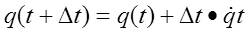 2. Fixed Interval Fourth-Order Runge-Kutta Method To improve the accuracy, Fourth-Order Runge-Kutta Method is used. The advantage of this method is that it does not require complex programming while still be able to increase the global error to fourth order. The implementation requires four evaluations per step: once at the initial point, twice at trial midpoints, and onces at a trial end point as following: 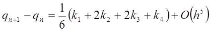 3. Variable interval Fourth-Order Runge-Kutta Method Apparently, the fixed interval Fourth-Order Runge-Kutta method has the disadvantage of using the same step size. Being able to adjusting the step size for further calculations will increase the flexibility as well as accuracy of the problem. Thus, variable interval Fourth-Order Runge-Kutta Method is also been implemented in the Matlab Code of this work. During the implementation of our Matlab Code, the best results are obtained by using the variable interval Fourth-Order Runge-Kutta Method. |
|||||
| Matlab codes Click to download 2D code Click to download 3D code |
|||||