|
ME
574 PROJECT |

|
||||
|
An
Axisymmetric
Model for Pore-Grain Boundary Separation |
|||||
|
|
|||||
|
Modeling |
|||||
|
|
|||||
| Mathmatical Modeling A pore located on a grain boundary. The pore size is characterized by r0, the radius of a sphere that has the same volume as the pore. The diameter of the axisymmetric unit is 2R, which represents pore spacing. It is assumed that the pore spacing is equal to the grain size for simplicity. A force fb at the outside edge of the interface represents the force on the interface by the grain boundaries. The pore moves by atomic diffusion on its surface, and the interface moves as atoms detach from grain II and attach to grain I. |
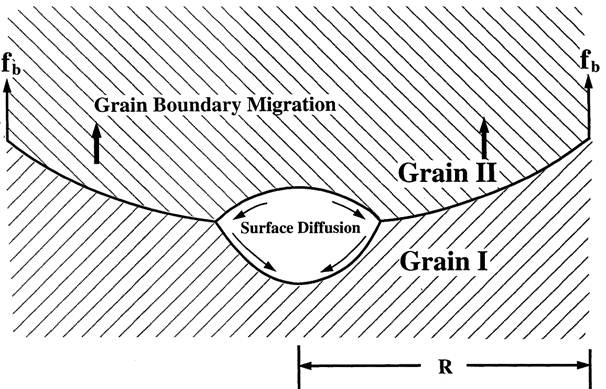 Figure 1. An 2D axisymmetric model. |
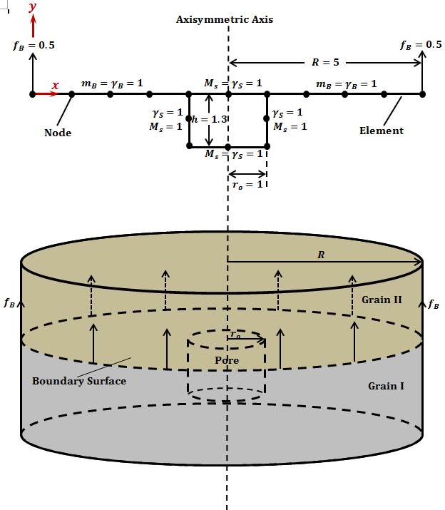 Figure 2. An 3D axisymmetric model. |
|||
|
Weak Statement |
|||||
| For
a system of surfaces and grain boundaries,
the total free evergy is G = gSAS + gBAB, where gS is the surface energy density, gB is the grain boundary energy density, AS is the area of the surface, AB and the total grain boundary area. After following methmatical procedure described in Yu et al., the virtual motion of the grain boundaries and surfaces change the total free energy by dG. 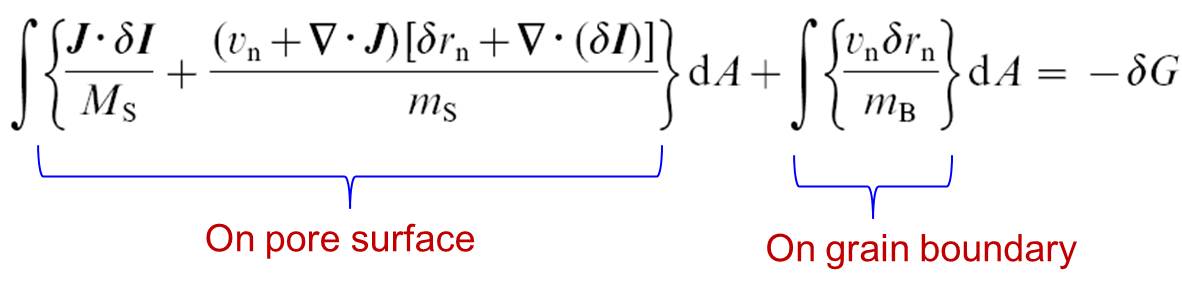 |
|||||
Finite
Element
Method 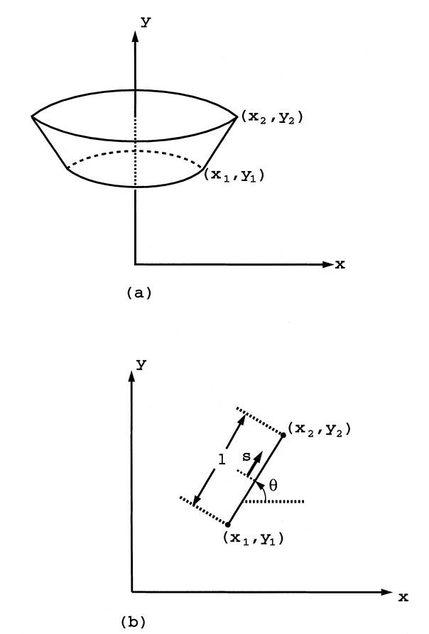 Figure 3. An axisymmetric element in three dimensions (a) and in a plane (b). |
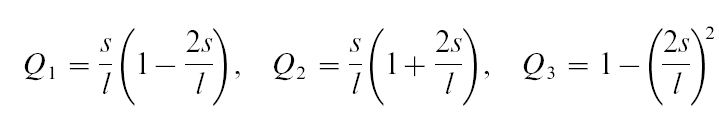
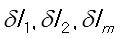
Figure 3 shows one element with nodes (x1, y1) and (x2, y2). The generalized velocities are 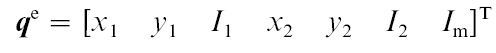 On the element, interpolate the virtual displacement and actual velocity linearly:  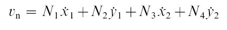 with
the interpolation coefficients being
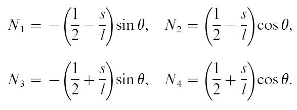  with
the interpolation coefficients being
 |
||||
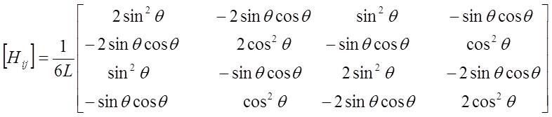
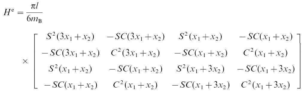
| H matrix The
FEM implementation of weak statement has been carried out for both 2D
formulation and axisymmetric 3D formulation. For
both cases, the viscosity matrix H on the grain boundary is a 4×4
matrix, and
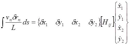
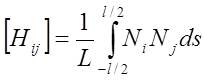
on the pore surface is 7×7 matrix. 1. 2D
formulation On
the grain boundary, the weak statement becomes:
Where
the viscosity matrix H is a 4×4 symmetric matrix calculated from:
On
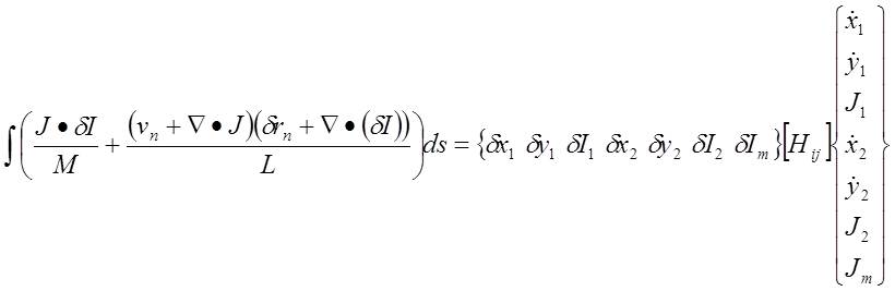
the pore surface the weak statement becomes:
This
will generate H as a 7×7 symmetric matrix. A Matlab code is
written to
automatically calculate the components of this viscosity matrix. 2. 3D
formulation The
derivation of the viscosity matrices for 3D axisymmetric case has the
same
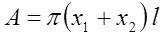
method as in 2D formulation. However, the integration now is not the
integration along the line. It becomes the integration over the area
the
rotated surface. For one element the surface area is:
The
difference can be seen when comparing this matrix and the one in 2D
case. The
7×7 symmetric viscosity matrix is also generated automatically by
a Matlab
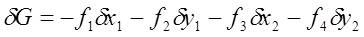
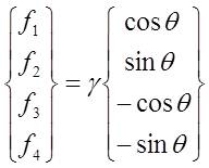
code. The
force vector for each element is derived from the right hand side of
the weak
statement. The free energy reduction of the element is: Using
the line element for 2D formulation, and axisymmetric
element for 3D formulation lead to two the
following corresponding force elements: 1. 2D
formulation
2. 3D
formulation There are only driving forces associated with
the movement of the coordinates. No driving forces are associated
with |
|||||
| Assembling 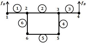 Figure 4. Model with minimum possible nodes and elements. |
In the preceding section, we showed how to obtain the local H and f matrices for each node on the grain boundaries and along the pore surfaces. In this section, we need to assemble the local H and f matrices to global ones so as to obtain the velocity of each node. In order to better understand how the assembling process looks like in the present problem, we start with the model containing the minimum possible nodes and elements, as shown in the Figure 4. Nodes 2,3 and 1,4 are called triple junctions and boundary nodes, respectively. In the following, the global H and f matrices are given by |
||||
Nodes 1 and 2 (element 1) 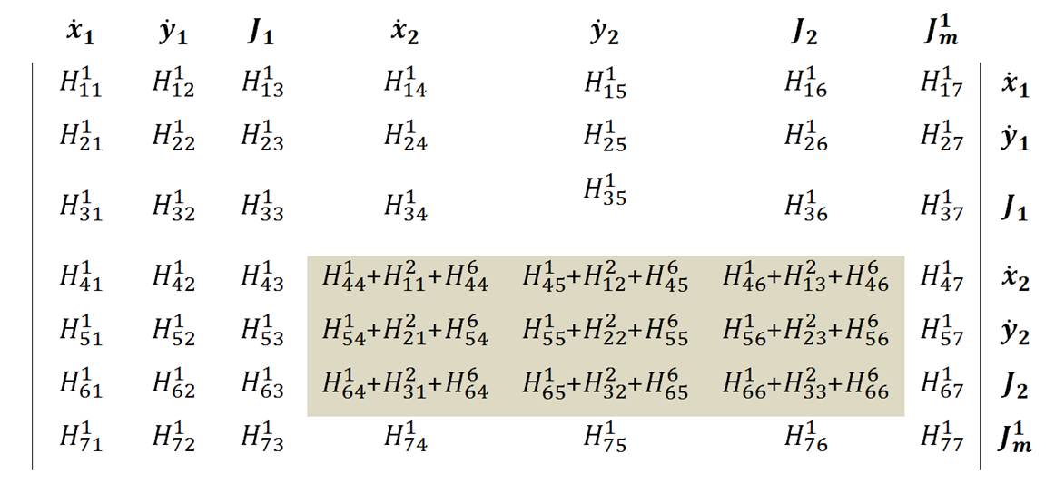 Nodes 2 and 3 (element 2) 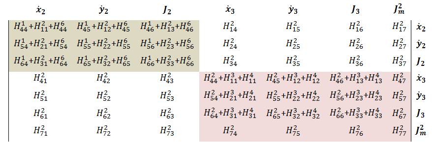 Nodes 3 and 4 (element 3) 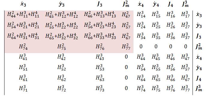 Nodes 3 and 5 (element 4) 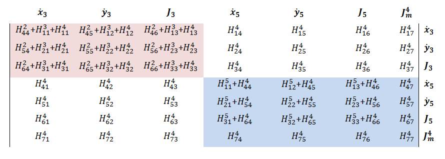 Nodes 5 and 6 (element 5) 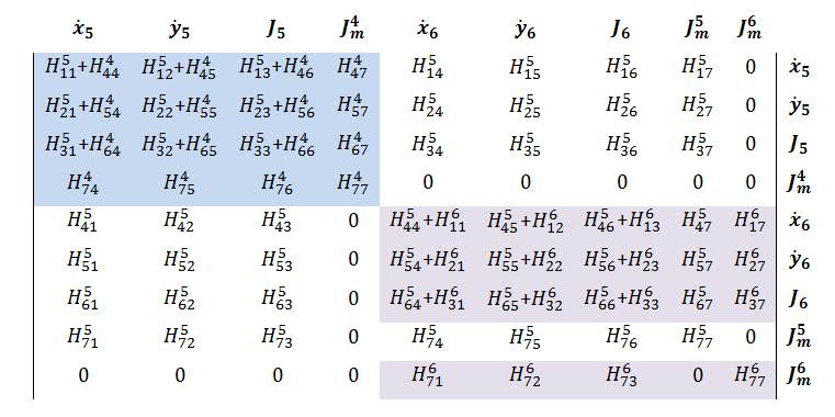 Nodes 6 and 2 (element 6) 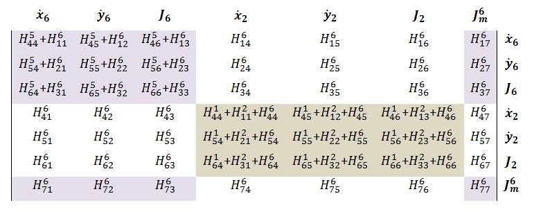 Big picture of the global H matrix is shown below. Off diagonal components is due to the triple junctions and the closed contour. 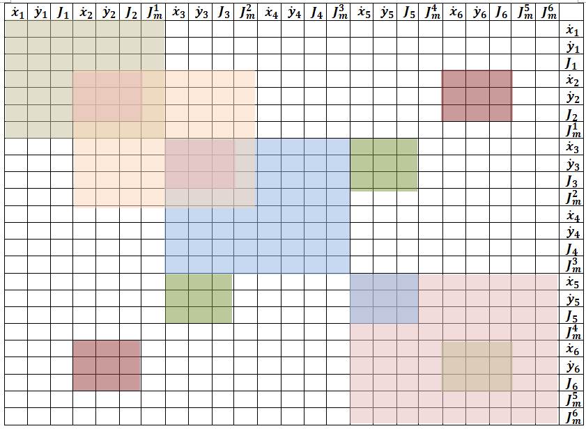 The global f matrix can be given by 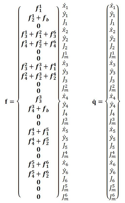 Inserting the above global H and f matrices into the following equation, a set of nonlinear ordinary differential equations governing the generalized coordinates as a function of time is obtained. 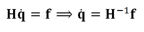 From the above equation, we can see that the velocity direction usually differs from the direction of the generalized force, i.e., gradient of free energy. The above equation is integrated numerically (i.e., Fourth-Order Runge-Kutta method) to evolve the surfaces. Boundary conditions At the boundry nodes 1 and 4, the velocity in the horizental direction is set to be zero. It can be done by adding a very large number to the corresponding H components of the boundary nodes. In addition, the external boundary force fB needs to be added to the corresponding f components of the boundary nodes, as shown in the preceding section. |
|||||
 .
.