PROGRAMMING
Building the global H-matrix
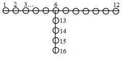
The thin film simulation with a grain boundary problem had some unique issues that needed to be resolved to accurately simulate the evolution with computer software. The method we used for numerical simulation was to number each of the points in the system as follows:
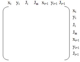
And the diffusion Local H matrix was of the form
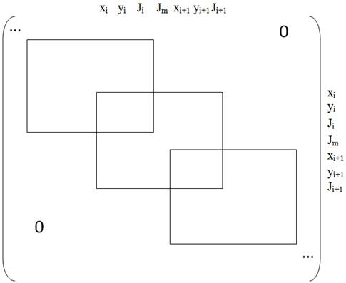
This allowed us to form a global H-matrix in the sequential order of the nodes, as calculated element by element. Each local H-matrix could be added into the global matrix as follows (local matrices for sequential boundary elements represented by the empty boxes):
This method allowed for the elements in both the surface of the thin film and the grain boundary to be contained in the same global H-matrix. The only element that wasn’t added in this method was the element connecting the grain boundary to the triple point on the surface boundary. In the figure above, this is the element connecting node 6 and node 13. Because 6 and 13 are not sequential nodes, the local H-matrix for the connecting element could not be added whole to the global H-matrix (like all of the other elements), but rather in 4 separate parts. The way in which we split the local H-matrix is shown below.
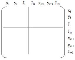
We split the 4 parts this way because this was how the elements were grouped together in the global matrix. We were able to take each of these 4 parts and add them individually to the global matrix according to their particular indices, as listed along the top and bottom of the local matrix in the figure above. Once we had finished this, the global H-matrix for the basic single film, single grain boundary problem was almost complete.
The final step was to fix the end points of the surface boundaries and fix the y component of the grain boundary node that was touching the ground. If this node were to move from the ground, it would be representative of a delamination, which is not what we are studying in this project. Therefore, we added 10^6 to the positions in the global H-matrix that were the locations of the x and y values for the endpoints of the surfaces, and to the y value of the node in contact with the ground. This caused these points to remain stationary in our simulations.
Completing the force vector was similar to creating the global H-matrix, summing the correct x and y force values in the correct vertical position based upon spacing using the same indices as used to compile the large matrix. Once we had both of these, we were able to compute a velocity vector, using the equation:
{v} = [H]^(-1) × {f}
We then used the velocity vector to update the position of all the nodes in the surface and grain boundaries.
For the multi-layer and multi-grain thin film simulations, the same principles were used as described above. Each element was added to the global H-matrix sequentially, and the elements that connected the triple points to the grain boundaries needed to be split into four parts and inserted into specific locations based upon the two nodes that comprised the endpoints of the particular connecting element. Several triple points were defined and stored after each iteration to track the evolution and position of the connections between the grain boundaries and the surface boundaries.
Checking element sizes
In order to ensure that calculation issues did not occur during simulation, the code needed to be able to resize the elements if one got too large or too small. To do this, the program ran a resizing loop that occurred immediately after the positions of the nodes were updated based on the evolution calculations.
If an element is found that is below the lower bound for element length, the program creates a new node at the bisecting point along the line of that element, and deletes the two original nodes that composed the element. That new point is then connected to the two points that were on the outside of the original nodes. This transforms three elements into two elements, completely deleting the element that was too small. Likewise, if an element is found to be beyond the bounds of the upper limit, a new node is created at the midpoint of that element, and the single element is split into two elements, half the length of the original.
Each time the resizing operation occurs, the index of the triple points needs to be updated so that the program knows where to find the location of the grain boundary connections. For instance, take a surface boundary vector with 10 points, and the triple point is the 5th node of this vector. If the 1st element is found to be too large in this vector, a new node is created in between the 1st and 2nd points, which leaves the boundary vector with 11 points. Also, the triple point is now the 6th node, rather than the 5th node. The opposite is true for the element deletion operation when an element is too small. Therefore, we had to make sure the program properly updated the triple point index every time an element was created or removed from a surface boundary vector.
Applying driving forces
The evolution of a thin film grain boundary has two main driving forces that we explored: the curvature of the surface, and the difference in surface tension which drives the bottom and top of the grain boundary. We had to artificially add the surface tension forces to our simulation. For the boundary point in contact with the ground, this was simple: we just added a force to the x component of the node that was connected to the ground. For the triple point connecting to the surface boundary, however, the addition was slightly different. To do this, we had the program set two different surface tensions for the same surface. For points to the right of a triple point, the surface tension was set higher than the surface tension of the points to the left of the triple point. This created a driving force at the top of our grain boundary, in addition to the simple force added at the bottom.