FINITE ELEMENT ANALYSIS
Interface Migration
In order to simulate the structure evolution through finite element analysis (FEA), the system is divided up into several “elements” connecting two “nodes” just as shown in FIGURE 1. This section discusses the procedures for analyzing interface migration through FEA. Later, the H matrices developed in this section are upgraded to take in account the concurrent effects of interface migration and diffusion.
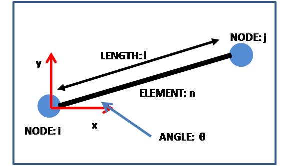
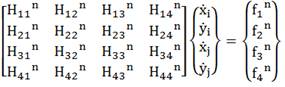
For an element “n” with end points “i” and “j” (displayed in FIGURE 1 above) the relationships between the positions and the velocities of the nodes, the length and the orientation of the element, and the forces on each node are described by the element’s local H matrix below:
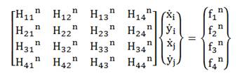
In each local matrix, each of the elements of the H matrix can be obtained through following equation:
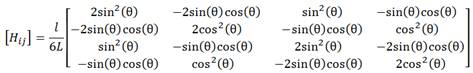
FIGURE 2: Schematics of 3-node, 2-element system discussed below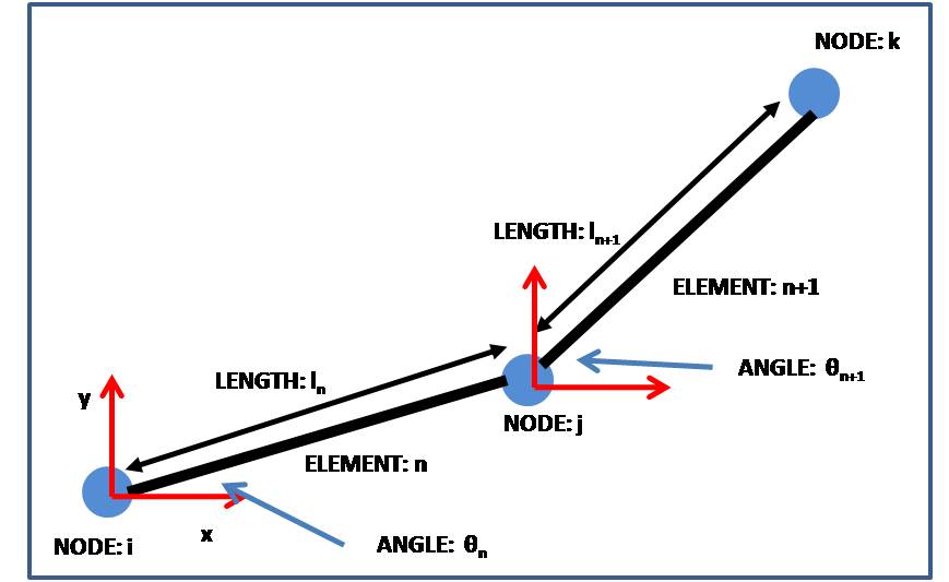
In order to model systems with multiple elements, local H matrices are assembled to create a global H matrix. When combining local H matrices, the global elements for the node(s) connecting multiple elements is calculated by summing up all the local elements (Hij) corresponding to the node. For instance, if the element “n” and element “n+1” are connected at the node “j”, the global H matrix element corresponding to the node j is the summation of Hij values corresponding to the node j in both local matrices for the elements “n” and “n+1”.
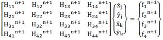
LOCAL H MATRIX FOR ELEMENT n:
LOCLA H MATRIX FOR ELEMENT n+1:
GLOBAL H MATRIX FOR THE SYSTEM CONSISTED BY ELEMENTS n AND n+1:
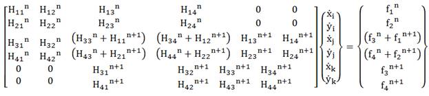
Since this particular system has three elements, dimension of the global H matrix is [6 x 6], and the 4 elements of the global H matrix (H33, H34, H43, and H44) – which corresponds to the node shared by the two elements – are obtained by adding the corresponding H matrix elements of both the element n and element n+1 local H matrices.
In addition, the dimension of the global H matrix for n-node (n-1 element) system is [2n x 2n] as each node contributes two rows and two columns (each row/column corresponding to x and y coordinate) for a 2D-system.
Concurrent interface migration and diffusion
In concurrent interface migration and diffusion, the local and global H matrices discussed in the simple interface migration problem are upgraded as the mass fluxes Ji and Jj (at each node i and node j, respectively) and the mass flux of the element m itself (Jm) are included. As a result, the dimension of each local H matrix is now [7 x 7] (instead of [4 x 4]), and the dimension of the global matrix for 3-node (2-ement) system is [11 x 11], 4-node (3-element) system is [15x15], and n-node (n-1 element) system is [(3n+n-1) x (3n + n-1)]. This is because each node contributes three rows and columns while each element contributes one row and one column to the global H matrix.

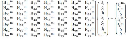
For the element “m” with end points “i” and “j”, now the effects of the mass fluxes at nodes “i” and “j” (Ji and Jj, respectively) and the mass flux of the element “m” (Jm) are taken into account. The following equation describes the structure evolution mechanism induced by concurrent interface migration and diffusion.
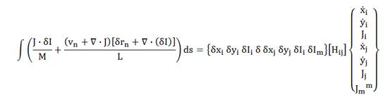
Where each local H matrix can be defined as follows:
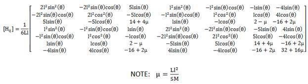
So for the element “m” with endpoints “I” and “j” – each having mass fluxes of Ji and Ji – and the element mass flux of Jm, the following equation can be used to relate the element and node configurations and the resulting forces and the velocities:
Finally, just as discussed in the sample interface migration problem, when assembling the global H matrix, the H matrix elements corresponding to the shared nodes’ x and y velocities as well as the mass flux at the node are calculated by adding up all the corresponding local Hij elements. As a result, (for a 2D-system) each junction between two elements results in 3 x 3 = 9 Hij elements that are obtained by adding up the corresponding local Hij values. More detailed calculation procedures taken in the project are described in the Programming page.