| Home | Introduction
| Approach & Model | Computational Process | Calculation of Electric Field | Results & Discussions | References & Appendix |
Approach & Model:
Details of the Nanotube System:
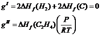
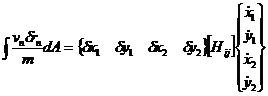
The reaction involved in
the nanotube formation is as follows:
![]()
where gaseous ethylene is decomposed to
form pure deposits of carbon on catalyst particles thus nucleating and forming
nanotubes. From this equation the free energy densities, gI and gII
for phase I and II respectively:
where DHf is the heat of formation of ethylene = 52.26kJ/mol
[Noggle], P is the partial pressure
of ethylene, R is the universal gas
constant, and T is the temperature in
K.
The surface energy was
estimated from the following equation:
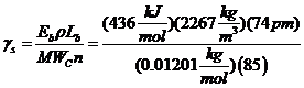
where
Eb is the C-C bond energy, ![]() is the nanotube density, Lb is the bond
length, and n is the average number of C atoms in the circumference of the
nanotube (10nm diameter in our case).
is the nanotube density, Lb is the bond
length, and n is the average number of C atoms in the circumference of the
nanotube (10nm diameter in our case).
The
permittivity of a carbon nanotube is difficult to predict since it depends on
the nanotube size, and band gap, but is reported to be in the range of![]() = 5 [Krupke et al.] so this value was adopted for
simulating the electric field.
= 5 [Krupke et al.] so this value was adopted for
simulating the electric field.
Theory and Finite Element Formulation:
The systems in which an interface is
separating a vapor phase, solid phase, and grains, it is often assumed that
vapor atoms diffuse so quickly compared to the rate of interface reaction such
as evaporation or condensation, which causes the vapor phase to have a
spatially uniform chemical potential at all times. This condition can be
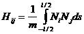
described by weak statement as follows,
![]()
Where, p represents the reduction in total free energy per unit interface area
moving per unit distance, ![]() is the magnitude of
interface displacement, m is the mobility of
interface, and G is the total free
energy of the system.
is the magnitude of
interface displacement, m is the mobility of
interface, and G is the total free
energy of the system.
Adopting the kinetic law stating that the
normal velocity of interface migration is proportional to the driving pressure p (![]() ), a weak statement
can be given as,
), a weak statement
can be given as,
![]()
The finite
element method determines an approximate normal velocity of interface that
satisfies a weak statement. In this work, an interface is modeled by an
assembly of straight line elements and followed the procedure given in Sun et
al to characterize linear geometries and seed the interface with nodal points.
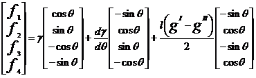
An assembly of straight line elements was
used to approximate an interface. Following figure shows one such element, on
the interface separating phase I and II. The positions of the two nodes, (x1,
y1,) and (x2, y2), fully specify the geometry
of the element.
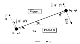
Figure: A
straight line element on an interface between phase I and II. When the element
undergoes virtual motions, the free energy varies, exerting on the two nodes
several forces: the axial force![]() , the torque
, the torque ![]() and the lateral force
and the lateral force ![]() . [Sun et al.]
. [Sun et al.]
Denote the
element length by ![]() and the slope by
and the slope by![]() ; they relate to the nodal positions as
; they relate to the nodal positions as ![]() and
and ![]() . The virtual motion of the interface relates to the virtual
motion of the nodal positions by
. The virtual motion of the interface relates to the virtual
motion of the nodal positions by
![]()
With the
interpolation coefficients being,
![]()
![]()
![]()
![]()
Here, s is
the distance measured on the element starting from the mid-point of the
element. Similarly, the interface velocity relates to the nodal velocities, ![]() ,
, ![]() ,
, ![]() and
and ![]() by,
by,
![]()
The variation of total
free energy associated with the virtual motion of single element is given as,
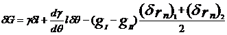
Express the
free energy variation in terms of virtual motions of the nodes:
![]()
Here![]() are the forces acting on the nodes by the element under
consideration.
are the forces acting on the nodes by the element under
consideration.
The left-hand side of
weak statement can be expressed in terms of variations of nodal positions,
velocities of nodal points, and angle theta,
Where [Hij] is a 4
x
4 symmetric matrix, also known as the viscosity matrix, is calculated from
Where N is a shape function
The forces on
each node were calculated from free energy variation, giving
-For the case of no electric field:
-For the case where
electric field is present:

Where, ![]() is electric energy density at the node
is electric energy density at the node![]() .
.
The force and viscosity matrices are then
assembled into a global matrix representing the contributing from all elements yield the general expression,
![]()
Then, the
velocities are then solved by using Gaussian elimination, and positions are
updated using Euler method. (See matlab code)
For a detailed
description of the technique used in the finite element method, refer to [Sun et al.].