|
SPATIAL ANALYSIS, ADVANCED TOPICS NRE501, SECTION 043 (3 credits) SCHOOL OF NATURAL RESOURCES AND ENVIRONMENT THE UNIVERSITY OF MICHIGAN http://www.umich.edu
|
|
SPATIAL ANALYSIS, ADVANCED TOPICS NRE501, SECTION 043 (3 credits) SCHOOL OF NATURAL RESOURCES AND ENVIRONMENT THE UNIVERSITY OF MICHIGAN http://www.umich.edu
|
|
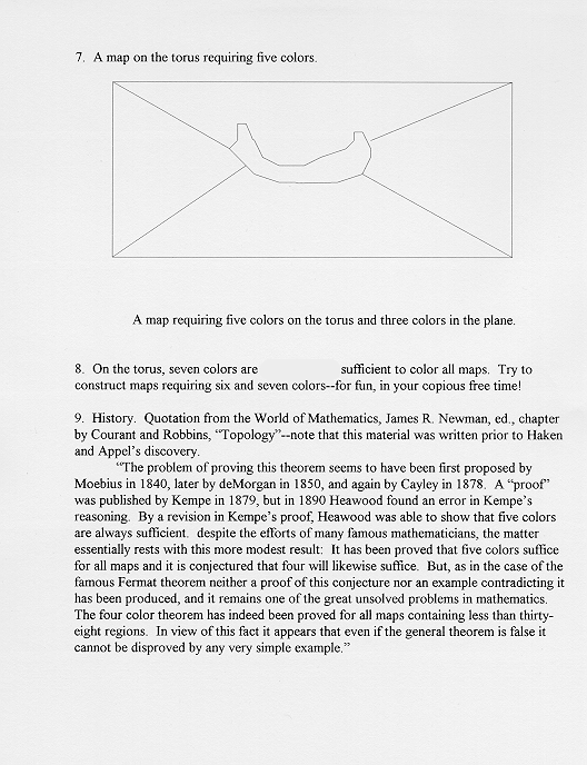
Professor Sandra Arlinghaus (Ph.D.)
Winter, 1999
Wednesdays, 6-9 p.m.
Office in Dana: 2044
Research office: 1130 Hill Street (Community
Systems
Foundation,
CSF)
Phone: 761-1357 (research office); 975-0246 (home,
call
between 9 a.m.
and 9 p.m.--phone with machine)
e-mail: sarhaus@umich.edu (preferred method of
communication)
Office Hours:
Monday (CSF), 10a.m.-1p.m.;
Thursday (CSF),
10a.m.
- 1p.m.
Wednesdays available much of the
day in
Dana.
Others by appointment. |
| This course offers students an opportunity to pursue advanced
spatial
topics related to their own interests. Students must bring their own
project
to this course (a chapter of a thesis, an ongoing project, or such). In
consultation with the instructor, students will be guided to
appropriate
tools, both theoretical and practical, that enable them to probe
various
spatial aspects of their project. As technology advances, so too must
an
understanding of the broad conceptual issues surrounding the
technology.
Class is informal lecture and discussion. |
Course Requirements
|
| MID-TERM PRESENTATIONS: Wednesday, March 10.
Party afterwards
at Sandy's home. FINAL PRESENTATIONS: Wednesday, April 28. Party afterwards at Sandy's home. |
| Overrides are required. Get an override from the
instructor.
Students should have some experience with mapping and should have a
project
in mind. All students will be required to have an active e-mail
account
at UM and an active web page. Students might wish to consider
enlarging
their ifs home directory space beyond the 10 mb default
allocation.
Class time will be spent in a combination of lecture on appropriate conceptual material and in a seminar/lab format dealing with student project concerns. It will be instructive for all students to hear the concerns of individuals and to see what sorts of issues are problematic and how they are addressed. All software used is for the PC. In using this website, note that material in table boxes is "official" material; all else is remnant or under construction material. |
![]()
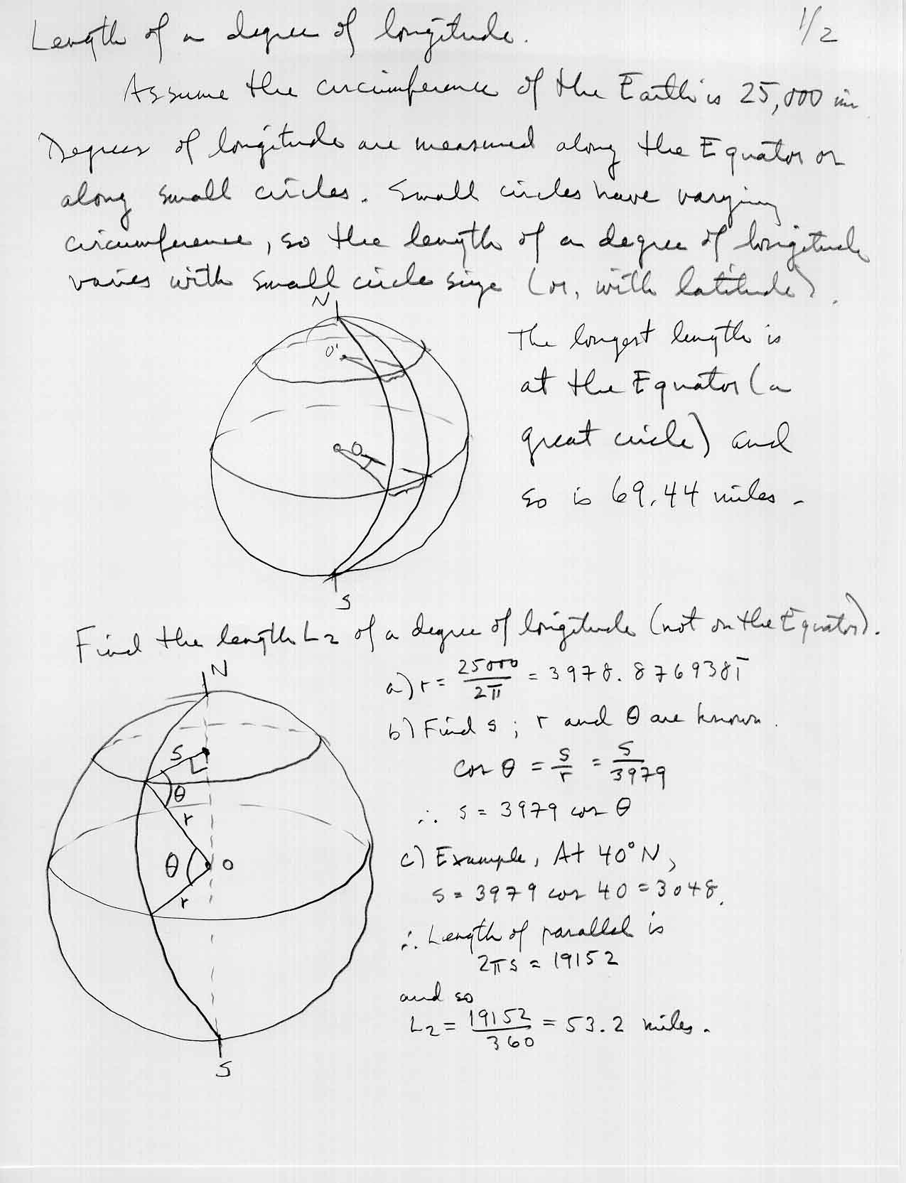
WEEK 1
Course mechanics
|
Web Page Creation--Basic Overview
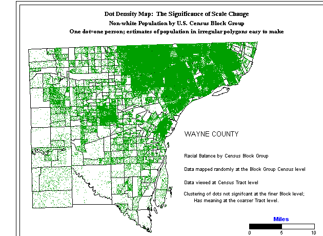
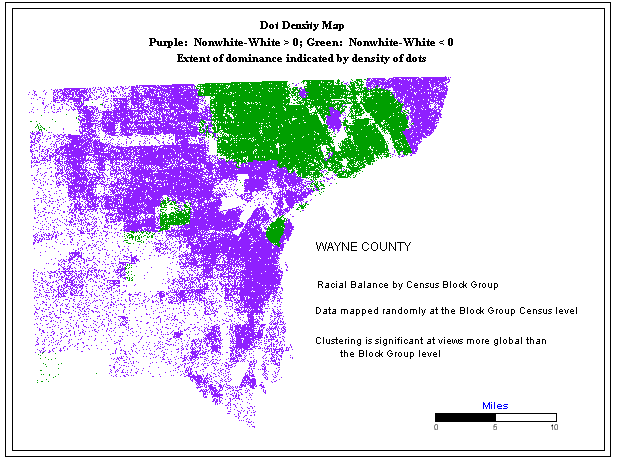
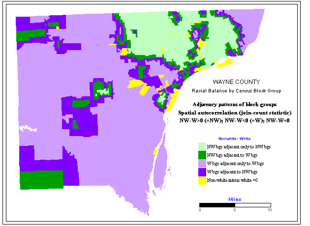
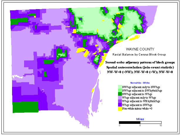
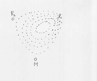
Within a Block Group, dots are scattered randomly. Thus, position of dots within the block group is meaningless. However, taking a smaller scale view, using Census Tracts, of the scatter at the Block Group scale, shows where there is clustering within a tract.
To pick out all block groups in which
Nonwhite
population dominates (layer test) To pick out all block groups in which
White
population dominates (layer test2) To pick out all block groups that are
touching
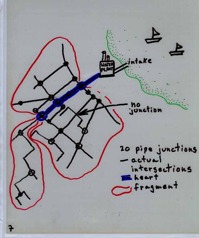
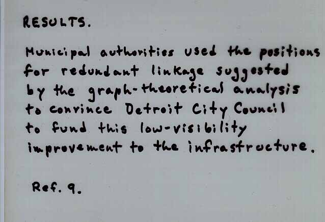
a dissimilar blockgroup: use test and test 2. Iteration of technique can produce a contouring of the region; also, weights can be introduced into the formulas. Graph-theoretic Background
Research Seminar/Lab Material |
![]()
WEEK 3
| Randomness, again:
diffusion of an
innovation
Measurement of diffusion: a conceptual approach based on the work of Torsten Hagerstrand Diffusion is a process in which anything that moves, or that can be moved, is spread through a space, from a source, until it is distributed throughout that space. How can diffusion be measured? One way is to trace the positions of things that are being diffused at different times. Torsten Hagerstrand, a Swedish geographer at the University of Lund, used the following technique to trace the diffusion of an innovation. The ‘thing’ being diffused (communicated) is an idea; the agents of diffusion, or carriers of new information, are human beings; the space in which the idea is to be diffused is a region of the world. Hagerstrand traces the diffusion process by imitating it with numbers. Such imitation, leading to prediction or forecasting of the pattern of diffusion, is called a simulation of diffusion. To follow the mechanics of this strategy, it is necessary only to understand the concepts of ordering the non-negative integers and of partitioning these numbers into disjoint sets. INITIAL SET-UP. In Figure 1 contains a map of an hypothetical region of the world. After one year, a number of individuals accept a particular innovation; their spatial distribution is shown in Figure 1. MAP BASED ON EMPIRICAL EVIDENCE--REGION INTERIOR IS SHADED
WHITE; CELLS
WITH NUMERALS IN THEM INDICATE NUMBER OF ACCEPTORS IN LOCAL
REGION.
Figure 1. Distribution of original acceptors of an innovation--after 1 year--based on empirical evidence. After Hagerstrand, p. 380. In Figure 2, a map of the same region shows the pattern of
acceptors
after two years--again, based on actual evidence. Notice that the
pattern
at a later time shows both spatial expansion and infill. These two
latter
concepts are enduring ones that appear over and over again in spatial
analysis---as
well as in planning at municipal and other levels.
Figure 2. Actual distribution of acceptors after two years. Might it have been possible to make an educated guess, from
Figure 1
alone, as to how the news of the innovation would spread? Could Figure
2 have been generated/predicted from Figure 1? The steps below will use
the grid in Figure 3 to assign random numbers to the grid in Figure 1,
producing Figure 4 as a simulated distribution, as opposed to the
actual
distribution of Figure 2, of acceptors after two years.
Articles on animated maps--scroll down on the attached site: www.imagenet.org CONCEPTUAL BASE Construction of the floating grid--the so-called "Mean Information Field" (MIF) Assumption: the frequency of social contact (migration) per square kilometer falls off (decays) rapidly with distance. Data from an empirical study: Units on axes: Definition: An area containing probabilities of receiving information from the central point of that region is called a mean information field, represented by Figure 3. To assign quantitites of four digit numbers to each cell in the MIF, it is necessary to use the curve derived from the empirical study (distance decay curve). It is used to
The size of the MIF is 25 by 25 kilometers squared. Observation is that the typical household moves no more than 12.5 kilometers. This field is then split into cells 5 by 5 kilometers squared. Assignment of probabilities From the graph of distance decay, a point 10 km from the center has a value of .167 associated with it. This is in households per square kilometer; there are 25 km squared in each cell; so the point value of the cell is 25*.0167=4.17. The center cell has a value of 110--an actual number of households. The total point value of all cells is 248.24--note the symmetry caused by assumptions about ease of movement in all directions outward from the center. Divide: 4.17/248.24=0.0168---so, assign 168 4 digit numbers to the cells that are 10 km from the center (two to the north, east, south, and west of center). Thus, the Mean Information Field is constructed. Some Basic Assumptions of the Simulation Method (Monte Carlo) Assumptions to create an unbiased gaming table:
Hagerstrand, Torsten. Innovation Diffusion as a Spatial
Process.
Translated by Allan Pred. Puu, Tonu. Mathematical Location and Land Use Theory. Springer-Verlag, 1997. Possibilities for Application Research Seminar/Lab Material |
|||||||||||||||||||||||||||||||||||||||||||||||||||||||||||||||||||||||||||||||||||||||||||||||||||||||||||||||||||||||||||||||||||||||||||||||||||||||||||||||||||||||||||||||||||||||||||||||||||||||||||||||||||||||||||||||||||||||||||||||||||||||||||||||||||||||||||||||||||||||||||||||||||||||||||||||||||||||||||||||||||||||||||||||||||||||||||||||||||||||||||||||||||||||||||||||||||||||||||||||||||||||||||||||||||||||||||||||||||||||||||||||||||||||||||||||||||||||||||||||||||||||||||||||||||||||||||||||||||||||||||||||||||||||||||||||||||||||||||||||||||||||||||||||||||||||||||||||||||||||||||||||||||||||||||||||||||||||||||||||||||||||||||||||||||||||||||||||||||||||||||||||||||||||||||||||||||||||||||||||||||||||||||||||||||||||||||||||||||||||||||||||||||||||||||||||||||
![]()
WEEK 4
Conceptual Material
|
![]()
WEEK 5
| Conceptual Material
-- refer
to articles on website URL given out in class.
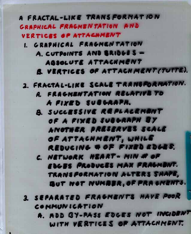
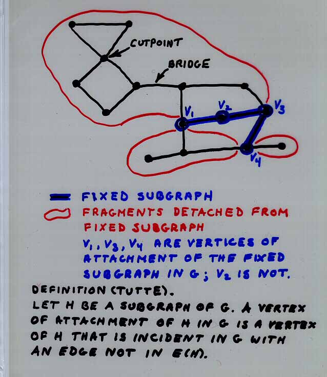
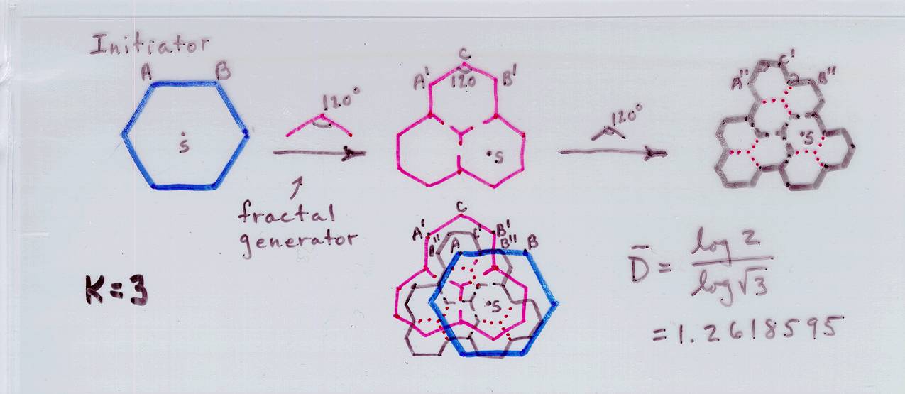
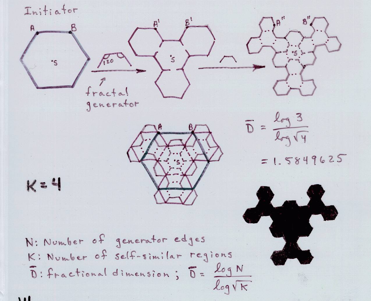
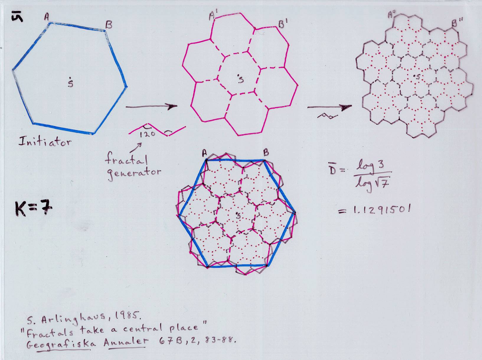
Fractal base
|
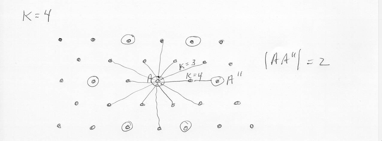
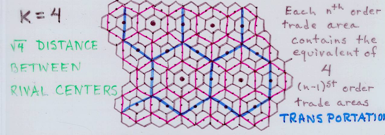
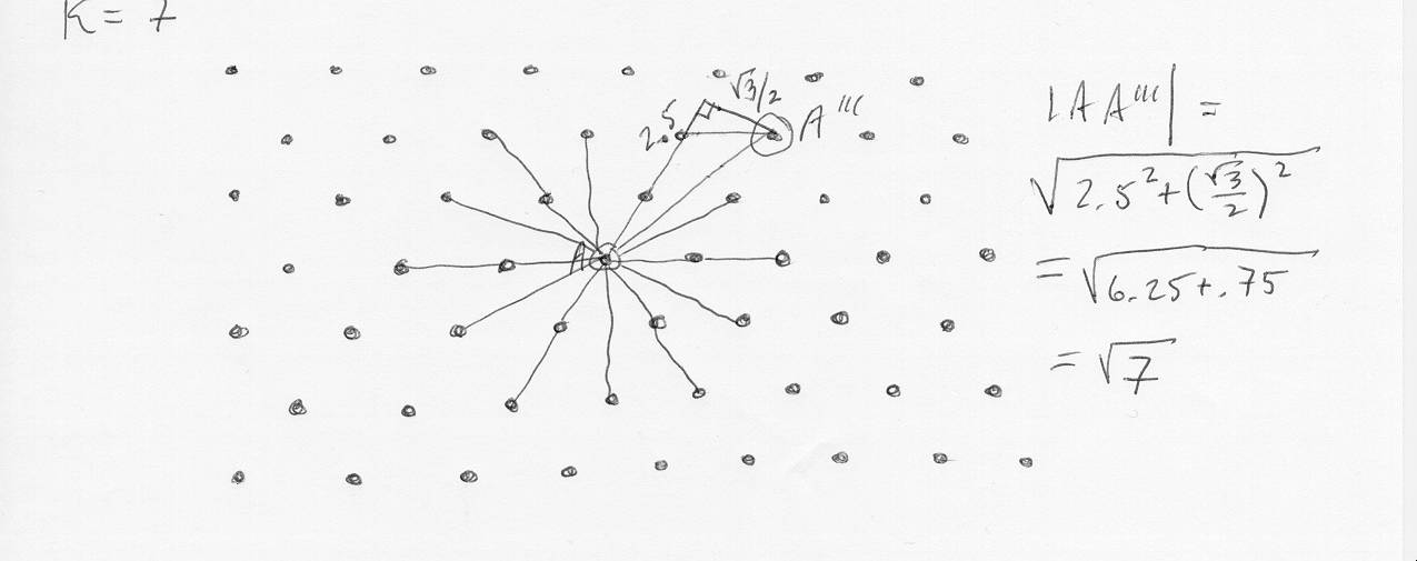
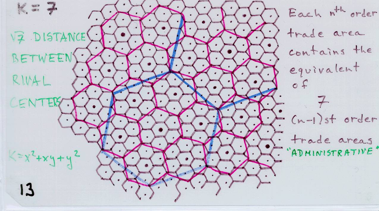
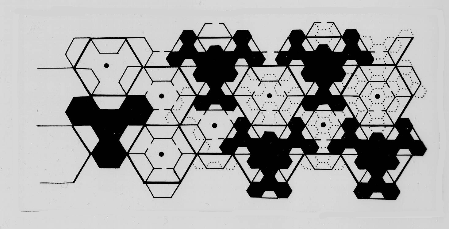
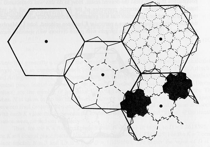
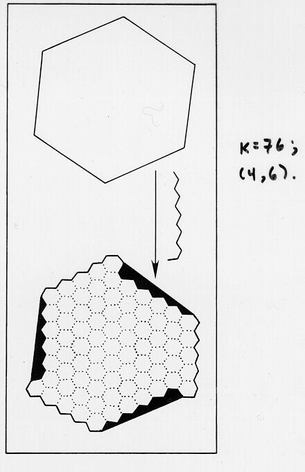
Conceptual Material:
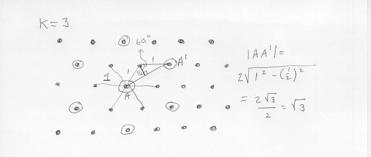
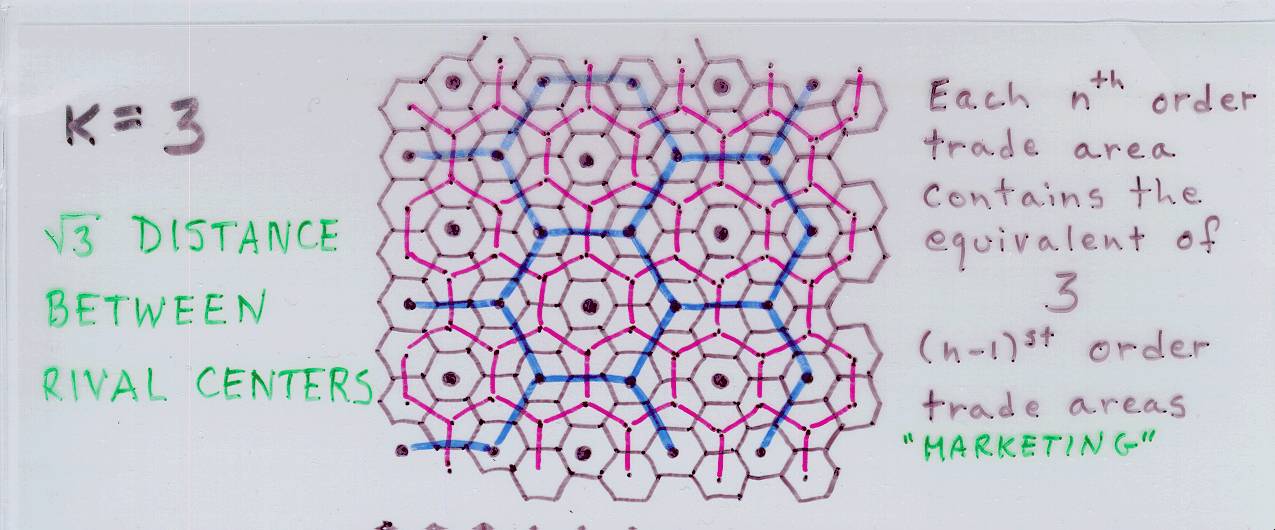
Centrality and
Hierarchy -- from the classical to the modern
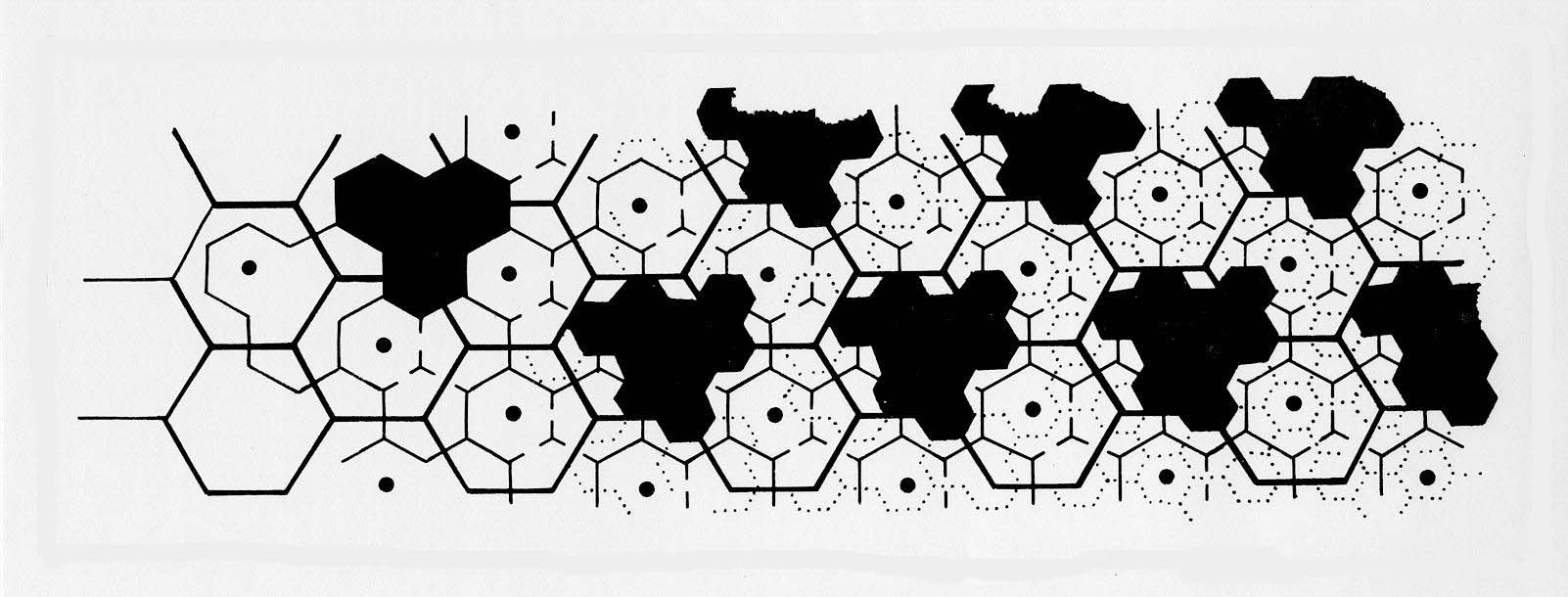
Christaller, Walter (books); Losch, August (book); Dacey, Michael (articles); Skinner, G. William (set of three articles); Marshall, John U. (article, Geographical Analysis); Arlinghaus, S. (article, Geografiska Annaler); Arlinghaus S. and Arlinghaus W. (article, Geographical Analysis); S. Arlinghaus, Electronic Geometry, (article, Geographical Review---reprints available). Related links--click to go to article linked to the website
of the Related map--partially digitized Christaller map. Research Seminar/Lab Material
Data Show and Overhead Laptop |
![]()
WEEK 7
Conceptual Material:
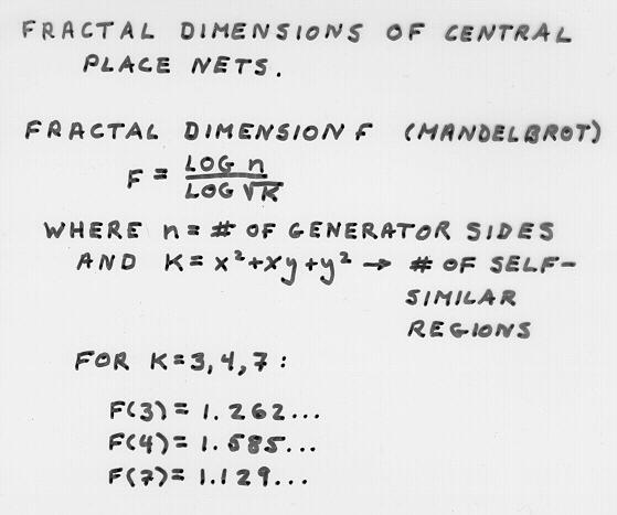
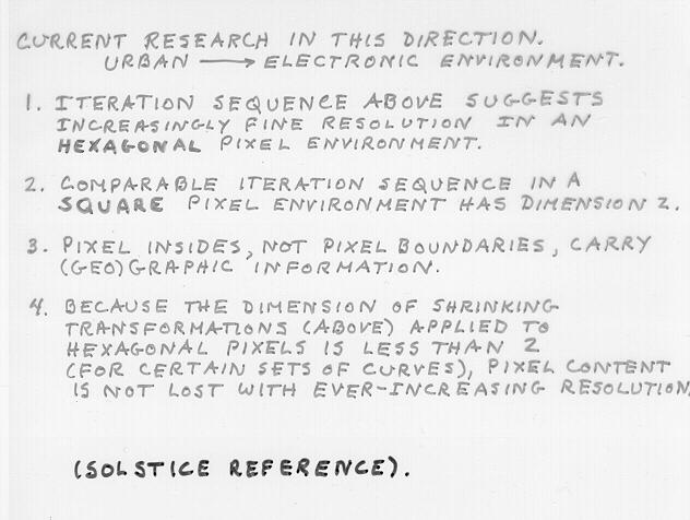
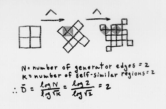
Hierarchy, Self-similarity,
and Fractals
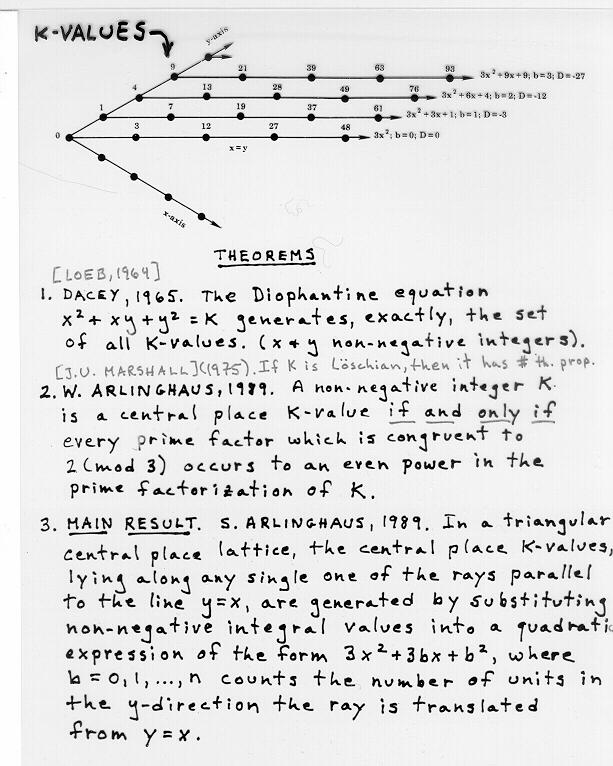
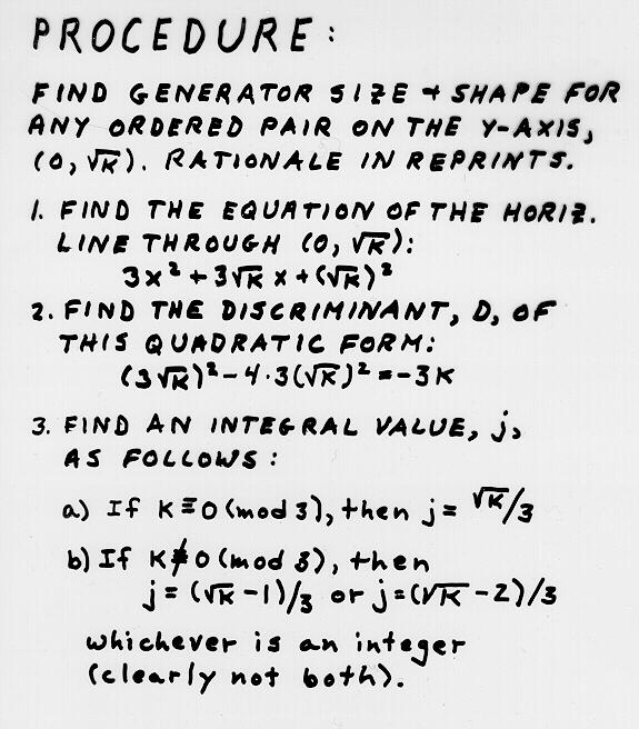
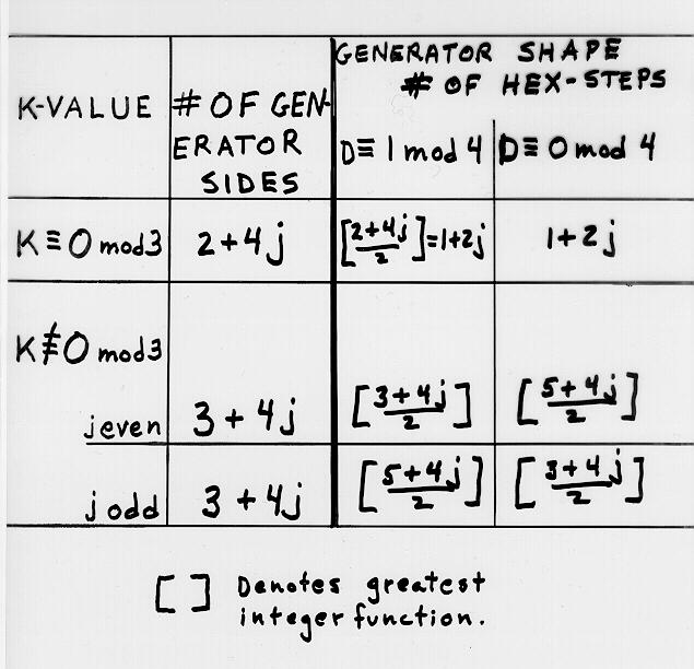
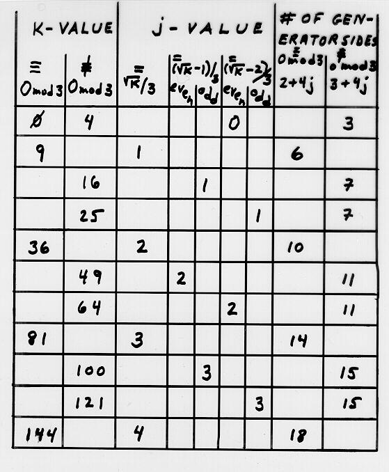
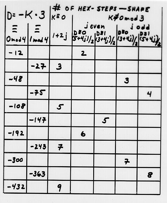
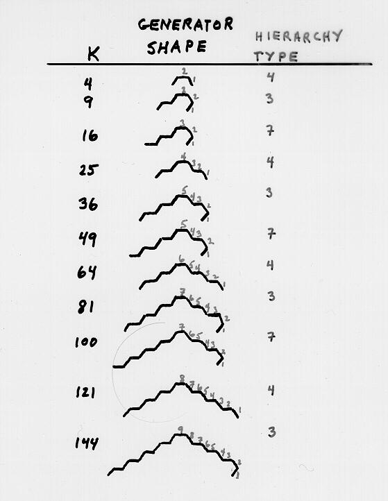
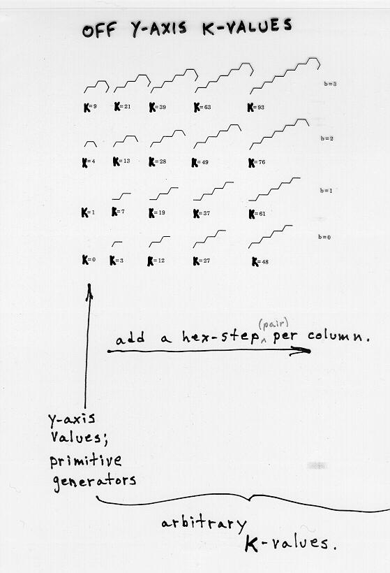
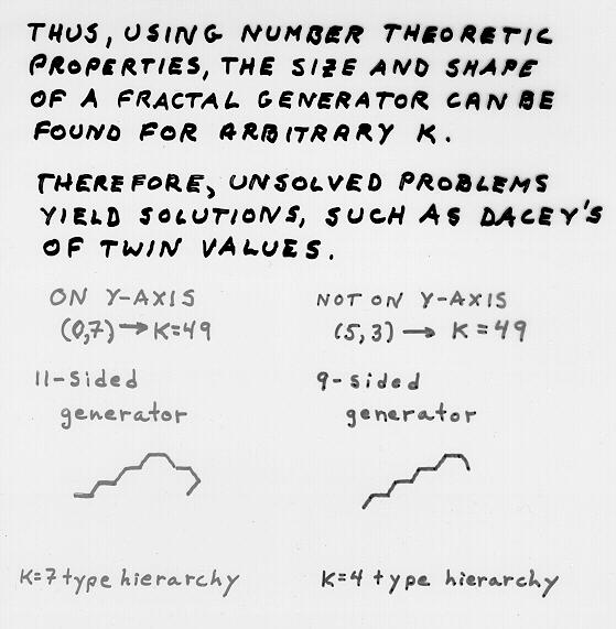
b. along lines parallel to the line y=x Statements of key theorems...all on Slide 18.
b. discriminant of the quadratic form c. the integral value, j, used to cross-cut the Diophantine equation. All on Slide 19.
centrality, hierarchy, scale, density, transformation, distance, orientation, geodesic, minimization, connection, adjacency Research Seminar/Lab Material
|
| Troubleshooting on an individualized basis. |
| Spring Break: February 27-March 8, 1999 |
| beiselt dkarwan feec gfiebich huangh jmeliker mbrush ninam schlossb zgocmen |
Conceptual Material:
Measuring Adjacency
WB: 24/159 * 100 = 15.1% BW: 24/159 * 100 = 15.1% BB: 44/159 * 100 = 27.7% WW+BB=69.8%; BW+WB=30.2%, similar regions are clustered. One might go on and on, but this is just a simple measure...divide the smaller by the larger--expect 1, get 0.43, here.
ArcView to Atlas GIS converter
1000*(1+.06/12)^12=1061.68 Compounded daily, you have at the end of a year: 1000*(1+.06/365)^365=1061.83 Flows other than money might exhibit a "compounding" effect. Generally, if P is the principal and i is the interest rate per period, at the end of period 1, interest earned is P*i and total amount is P+P*i=P(1+i) at the end of period 2, interest earned is the principal
times the
interest rate, but now the principal is the total amount (the
compounding
effect) from the end of period 1, or P(1+i)i. The total amount is
the principal plus the interest or
|
Conceptual Material
Individualized web work; mapping; other, as needed. |
WEEK 12
| Conceptual Material
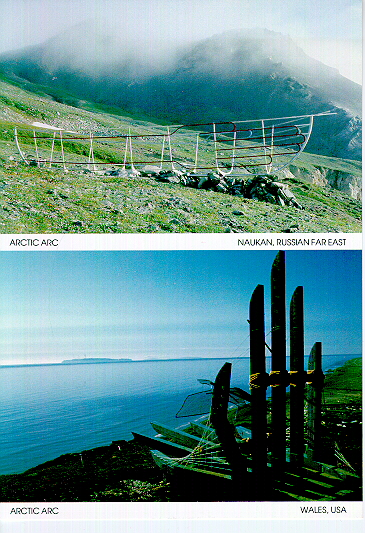
With map projections, the challenge is to choose a projection whose favorable qualities match the aspects of the map that you wish to emphasize. The same basic strategy applies when mapping in real-world situations and particularly in harsh environments. MAPPING AND REAL-WORLD APPLICATIONS:
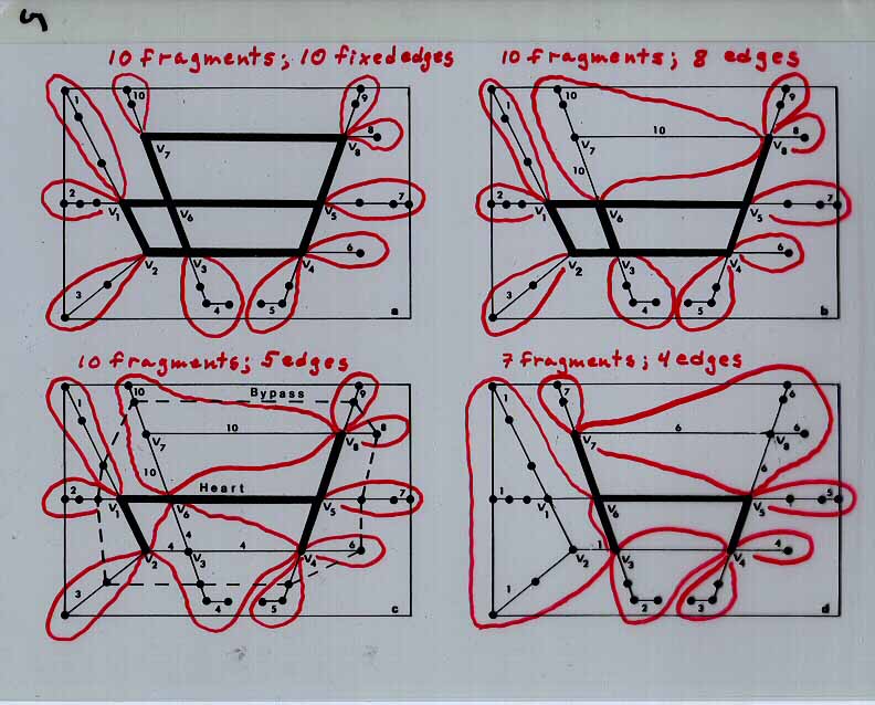
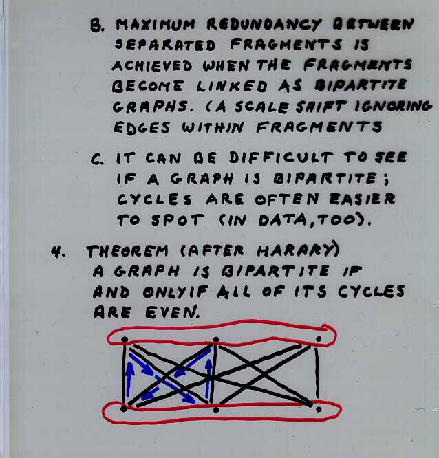
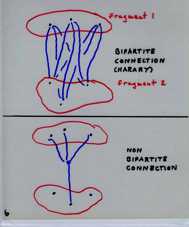
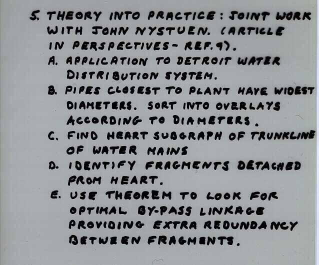
Per Hage and Frank Harary, Island Networks, Communication, Kinship, and Classification Structures in Ceaniia, 1996, Cambridge University Press. Per Hage and Frank Harary, Exchange in Oceania, A Graph Theoretic Analysis, 1991, Oxford University Press.
2. Grabbing an image a. request permission to use and behave according to answer to request; b. give cutoff date; c. put in own directory to avoid bandwidth drain d. cite source 3. Do not use an image if there are disclaimers on it; 4. U.S. Government materials; these do not generally require written requests for printed materials...so, apparently, use them...cite source and so forth and send a request if it indicates that one should be sent. 5. Link to search engines...do not inform them. Cite them: "here's what Yahoo says about Leelanau...", copy link and paste...pass along your search skills...can increase traffic on your site. 6. I will assemble all of it and make CDs for each. Check out security issues and let me know. 7. Citation of software and electronic sources: get citation from metadata--give links to websites. 8. Student UM accounts can be kept past graduation (contact Alumni Association) 9. Outside US copyright and related laws/ethics vary. 10. Citations...be clear as to what kind of material is being cited--maybe one category for hardcopy, one for software. 11. Concepts...tie to spatial concepts...broad connections send broad message: centrality, hierarchy, scale, density, transformation, distance, orientation, geodesic, minimization, connection, adjacency to name a few. |
| Conceptual Material
IMPLEMENTING PROJECTS
Troubleshooting on an individual basis. DOS commands for zipping and unzipping files using PKZIP 204G (both on a single diskette and on a sequence of diskettes). PKZIP 204G files are in my Public Directory, in the PKZIP folder. |
![]()
WEEK 14
| Conceptual Material
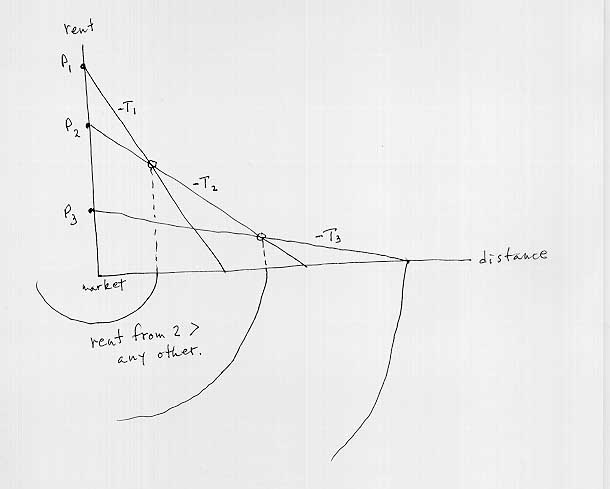
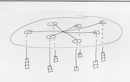
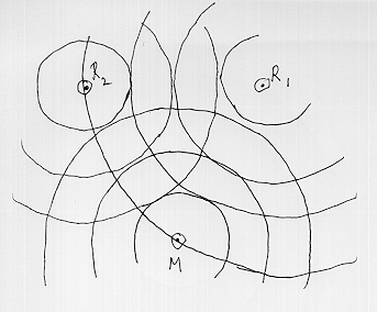
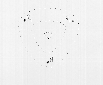
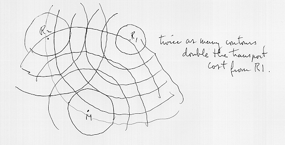
SELECTED MODELS, TRANSPORT COST, LOCATION, AND CONTOURING
c represents production costs d is distance to market t is transport rate (hence, dt is total transport cost)
T = Yt,
R = P2 - T2 d R = P3 - T3 d
Weber, Alfred. Alfred Weber's Theory of the Location of Industries, trans. C. J. Friedrich. Chicago: The University of Chicago Press, 1928. Textbooks (out of print; contact instructor)
|
| zgocmen schlossb ninam mbrush jmeliker huangh gfiebich feec dkarwan beiselt |

