ME 574: Nano/Microstructural Evolution

Theory of Interface Migration and Numerical Simulation

Weak statement used in our simulations:

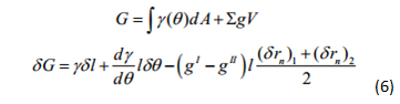
Let us consider a solid particle of random shape which is in contact with its vapor. This particle is shown in Figure 1. The solid particle can be composed of a number of nodes as shown. The two dimensional (2D) meshing of the particle determines the level of accuracy of its numerical simulations. In order to mathematically express the shape change associated with the particle as a result of interface migration we derive an expression for the driving pressure 'P' by linking virtual migration and the Gibbs free energy of the system, shown by equation 1.

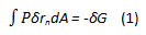
Where δ_rn describes the small change of distance in the normal direction to the surface and – δG describes the reduction in Gibbs free energy of the system. From the kinetic law we may link the driving pressure to the normal velocity as shown in equation 2. Here 'L' describes the mobility of the particle interface.

Substituting (2) into (1), we arrive at the weak statement used for our numerical simulations of interface migration as shown by equation 3.

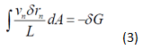
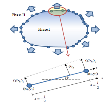
Figure 1: Interface migration of a random solid particle. A single element of the particle has been described in detail.

Mathematical modeling of a single element:

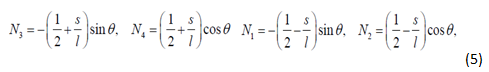
In order to model the system shown in Figure 1, we divide the particle into a number of elements. One such element has been enhanced in the figure for explanation. Along with the x and y coordinates we introduce a 's' coordinate system to describe the length 'l' of the element. Now, δr_n of the element can be expressed as a function of δr_n1 and δr_n2 , which can be further expressed in terms of δ_x1 , δ_y1, δ_x2 and δ_y2 , where (x₁,y₁) and (x₂,y₂) are the coordinates for the two nodes of the element. Equation 4 shows this expression. Here N₁, N₂, N₃ and N₄ when solved for turn out to be functions of a variable 's' and constants 'l' and 'θ' (equation 5).

Using (4) we can easily derive the normal velocity v_n=δ_rn/δ_t. From (3), integrating these parameters over the area (or volume in the case of 3D problems) we get the left hand side (LHS) of our weak statement.

To describe the reduction in free energy of the system, we use the fundamental expression for free energy of a system from non-equilibrium thermodynamics shown in equation 6.

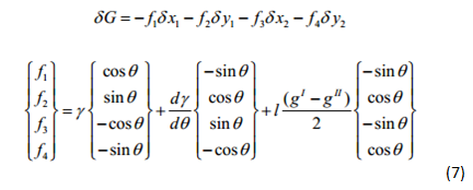
We may also represent δG as a function of four conceptual forces f₁,f₂,f₃ and f₄ acting at the two nodes of the element, equation (7). These forces multiplied by the incremental x, y distances give the negative work done to the system. Forces f_1-4 are also expressed in matrix equation form. Here γ is the surface energy per unit area that tends to shrink the element, dγ/dθ is the torque that tends to rotate the element and (g^I -g^II) represents the difference in free energies due to phase transition.

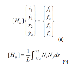
Solving the weak statement (3) we get a matrix equation relating the velocities of the two nodes in the x and y directions to the forces in those directions, equation (8). The [H_ij] matrix is the relation factor and can be expressed by equation (9). It is to be noted that the elemental H matrix (also called the local matrix) is a 4x4 axi-symmetric matrix and can be computed for a given element given its parameters and the mobility.

Novelty of our code:

Generation of the [H_ij] matrix for each element can be done by manually calculating each of its elements. This would however surmount to highly inefficient coding and limitations with regard to number of elements in a given simulation. In order to allow for a large (and random) number of elements in a given system, we introduced an automated approach to the generation of these local matrices. A snapshot of the MATLAB code block implementing this feature is shown in Figure 2. Function 'func1' returns the corresponding expressions for N_i and N_j (i and j varying from 1-4) as shown in (5). The 'quad' function then integrates the product over the limits (–l/2) to (l/2) to obtain what is shown in (9).

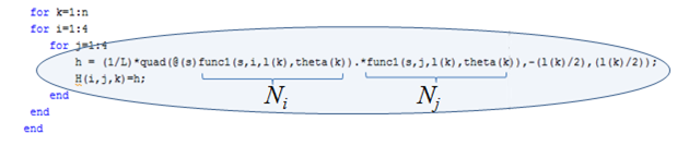
Figure 2: MATLAB code block for automated [H_ij] local matrix calculation.

This automated approach proves vital to improving the overall efficiency of our code and removes any limitation with respect to the degree of meshing for the system.

The local H matrices for the elements are then assembled into a global H-matrix as shown in Figure 3. As seen in the figure the assembling mostly follows an organized pattern with the quadrants for the last element H-matrix being spread between the four vertices of the global matrix. This scheme of assembling applies to closed surfaces only and may vary for other type of surfaces. For a system with 'n' number of nodes the global H-Matrix is a 2nx2n matrix. Also the F matrix for the system is a 2nx1 column vector.

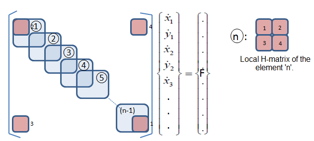
Figure 3: Global H-Matrix generation for the system.

Taking the inverse of the global H matrix and multiplying it with the F-matrix, we get the velocities column vector shown in Figure 3. A suitably chosen time step can then be multiplied with these velocities to obtain the incremental distance moved by the nodes in the x and y direction. The x and y coordinates can thus be updated after each time step for the duration of the simulation. Thus we can numerically simulate the particle evolution due to interface migration over time.

Numerical Implementation of the Intersection Calculation

Assumptions

1) Two particles are approximately convex polygons.

2) The number of intersections of the two particles is either 0 or 2.

Ideal Solution

Detect the intersections between all possible pairs of lines which make up the particles.

Process to detect the intersections and form the combined particle

Function [intsctFlag CombineShapeMatrix] = DetectIntersectionPolygons(Matrix1,Matrix2) "intsctFlag" : value=1 indicating two polygon intersected. Value =0 indicating no intersection "CombineShapeMatrix]" : if they intersect, return new matrix stored all points of combined shape in counter clockwise order; if NOT, return empty vector.

1. Rotate the coordinates onto the horizontal axis according to θ.

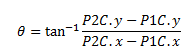
The horizontal axis will provide convenience in identifying relative positions.

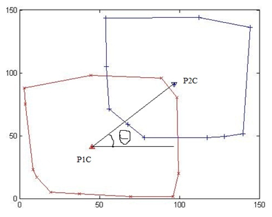
Figure 4

2. Identify all candidates' pairs of lines.

Here, a simple policy is used to identify candidates.

PL: the polygon whose center is on the left (has smaller x-value). (Red one in Figure 5)

PR: the polygon whose center is on the right (has larger x-value). (Blue one in Figure 5)

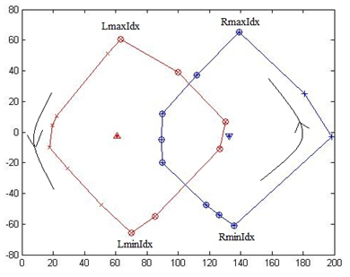
Figure 5

LmaxIdx: point has largest y-value in left polygon. Lminidx: point has smallest y-value in the left polygon.

RmaxIdx: point has largest y-value in the right polygon. RminIdx: point has smallest y-value in the right polygon.

Since all points on the polygon is stored in a counter clockwise order.

PLrightPoint: set of points in the right side of left polygon (denoted as red circle in Figure 5)

PLrightPoint can be built as starting from LminIdx, add increasing idx with mod ( idx= max([mod(idx+1,length(PL)) 1]) ) until LmaxIdx.

PRleftPoint: set of points in the left side of right polygon (denoted as the blue circle in Figure 5)

PRleftPoint can be built as starting from RmaxIdx, add increasing idx with mod (idx = max([mod(idx+1,length(PR)) 1]) ) until RminIdx.

3. Detect all intersections between pairs of lines.

Fix "Line" in left polygon, test all "TestLine" in the right polygon to see whether they have an intersection or not.

MATLAB has the function "polyxpoly" which returns the coordinates of intersection between two lines if they have one or returns an empty vector if they do not.

Line = [PLrightPoint(idx) PLrightPoint(idx+1)], while
TestLine = [PRleftPoint(Ridx) PRleftPoint(Ridx+1)]

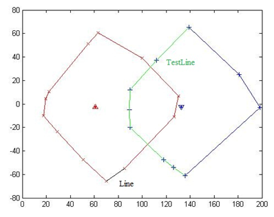
Figure 6

As shown in Figure 6, fix 1st "Line" (denoting as the black line in left polygon), test all "TestLine" (denoting as the green lines in the right polygon). All "TestLine" do not intersect with "Line".

As shown in Figure 7, fix 2nd "Line", test all "TestLine". There is one "TestLine" has intersection with "Line", store the coordinates of this intersection (denoting as the magenta circle) in the vector IntersectionPoint.

As shown in Figure 8, fix 3rd "Line" (denoting as the black line in left polygon), test all "TestLine" (denoting as the green lines in the right polygon). All "TestLine" do not intersect with "Line".

As shown in Figure 9, fix 4th "Line", test all "TestLine". There is one "TestLine" has intersection with "Line", add the coordinates of this intersection (denoting as the magenta circle) in the vector IntersectionPoint.

As shown in Figure 10, fix 5th "Line" (denoting as the black line in left polygon), test all "TestLine" (denoting as the green lines in the right polygon). All "TestLine" do not intersect with "Line".

Up to now, all intersections are detected and the coordinates are stored in the vector IntersectionPoint.

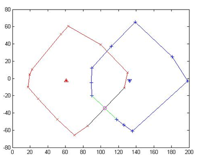
Figure 7

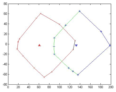
Figure 8

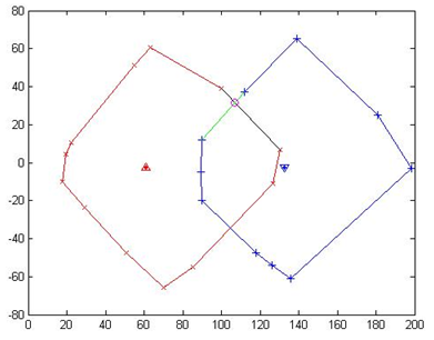
Figure 9

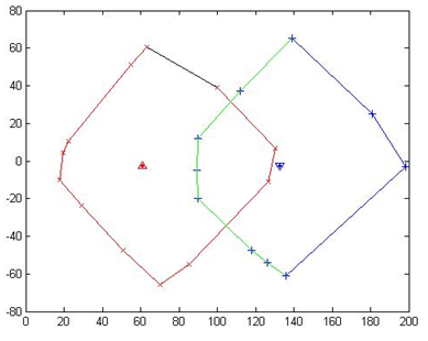
Figure 10

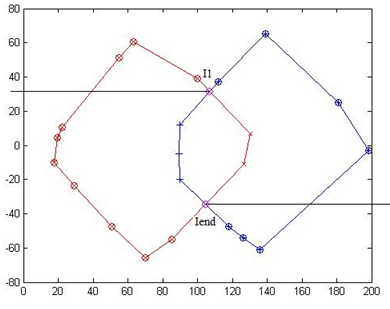
Figure 11

4. BuildNewShape

call function [CombineShape PLIDX PRIDX] = BuildNewShape(PL,PR,IntersectionPoint)

Where PL is the left polygon, PR is the right polygon, and CombineShape is the counter clockwise ordered points representing the merged particle.

PLIDX: indices of points previously belonging to the left polygon and currently belong to the new merged shape

PRIDX: indices of points previously belonging to the right polygon and currently belonging to the new merged shape

As shown in Figure 11, all points belonging to merged particle have special relative coordinates.

PL(PLIDX): points of new merged particle from left polygon has one of the following two criterias:

LeftIdx∈PLIDX

1) PL(LeftIdx).y > I1.y (I1 is the intersection with larger y-value see Figure 11)

2) PL(LeftIdx).y < I1.y && PL(LeftIdx).x < Iend.x (Iend is the intersection with the smaller y-value see Figure 11)

And # of items in PLIDX <= # of points of left polygon.

A similar operation is conducted for PRIDX, "CombineShape" stores the actual coordinates of all points belonging to the merged shape according to PLIDX and PRIDX. The order of the new merged particle is shown in Figure 12.

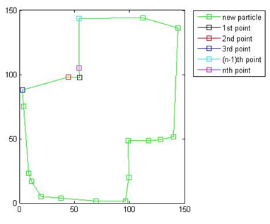
Figure 12

As shown in Figure 12:

I1": coordinates of intersection with larger y-value.

"Iend": coordinates of intersection with smaller y-value.

CombineShape = [I1 PL(PLIDX) Iend PR(PRIDX)]

5. Rotate back to original axis

The final result is shown in Figure 13.

If the two polygons do not have any intersections, return intsctFlag=0 CombineShapeMatrix=[] as shown in Figure 14.

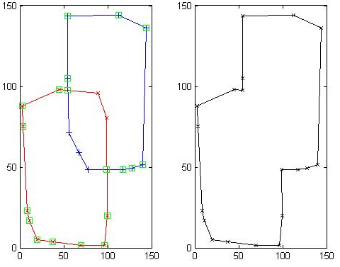
Figure 13

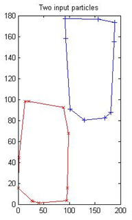
Figure 14

Highlights

1) Inputs take arbitrary convex polygons.

2) The relative positions of the two polygons can be arbitrary.

3) Does not matter how many points of one polygon are contained within the other polygon, since the basic idea of this detection is to test the pairs of lines instead of testing the points.

Function Dependence

test.m: main file used to randomly generate two convex polygons and test intersection.

DetectIntersectionPolygons.m: function used to find intersection

Convert2PlotFormat.m : used in DetectIntersectionPolygons.m to convert the matrix format(store an n-point polygon with 2-by-n matrix with row 1 for x-axis and row 2 to y-axis) to plot format (using complex number to denote the x-y coordinates and directly apply to command "plot").

BuildNewShape.m: used in DetectintersectionPolygons.m to build new merged polygon.