Simulation

Mesh:

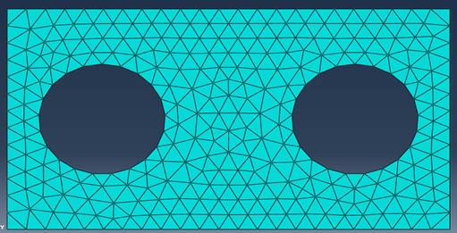
Figure1: Final Mesh Visualization 
ABAQUS is used to generate 2D meshing which consists of small triangles.
Since mesh can provide a lot of important information to a simulation, a good mesh is indispensible. Usually the following information is provided:

1. The number of each element;
2. The numbers of three nodes in one element;
3. Coordinates of all the nodes;
4. The number of nodes which are on special positions, such as boundaries and forces applied areas;

In this specific problem, the numbers of the nodes on voids’ boundaries are also needed.
Effects of stress field:
In step 3, H matrix and F matrix are constructed to calculate the velocity of nodes on voids’ boundary at different time. The stress field can affect strain energy of different node, which will change F matrix and change the velocity finally. The relationship is shown below:

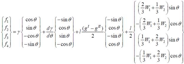
Where W1 and W2 terms are strain energy.
The governing equation in stress field simulation is:

Where  is a stiffness matrix, F is force matrix and d is displacement matrix.

Considering the significant effect of interaction between two voids on strain energy, simulation is conducted to calculate strain energy at different time. In this project, linear shape functions are used to describe stress field. The detailed Matlab code is put at the end of this report. A displacement profile at a time is shown below:

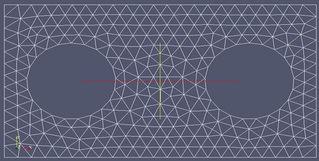
Figure 2: Original displacement profile

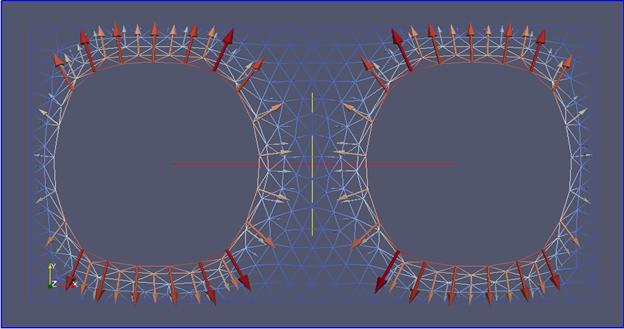
Figure3: Displacement profile at the very beginning of simulation

If displacement profile is known, the following equation can be used to calculate strain energy at different nodes:

Where Ui’j is strain and Cijkl is 2D stiffness matrix.

Assembly of H and F Matrix

Assemble contributions from all elements. Starting with a global H matrix with all zero elements and count all the elements eachlocal h matrix, and add them to the correct locations in the global H matrix. Below shows the format of one element

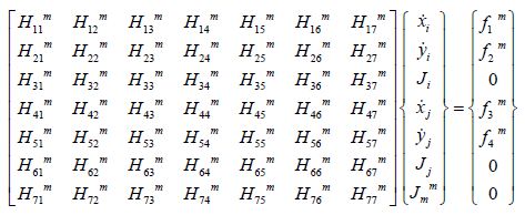
Below shows a part of the global H matrix, vn column and force column. Each of h matrix are assembled into the global H matrix. The last node is connected with the first node, so it should be taken care specially. Similary, F matrix can be assmled.

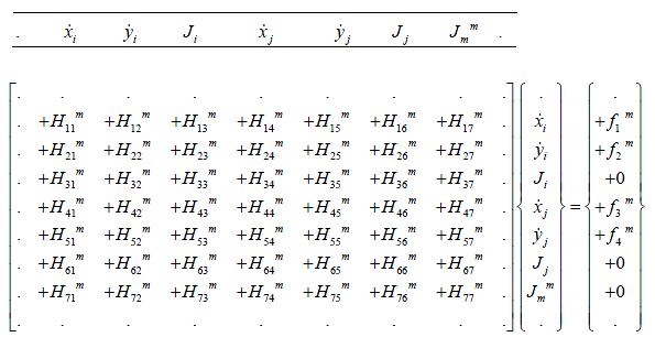
Once H and F are ready, V can be calculated by V=H\F. Then by setting a step time d_t, the displacement of each node can be calculated. Once new coordinates are obtained, the same cycle repeart again and again.

Difficulties in Simulation:
This simulation is a dynamic process, in which stability cannot be ignored. Time step is critical to stability. Usually a tiny step time can provide an accurate and stable simulation, but time cost is large. In future a code with step time adjusting feature is necessary. If result can converge, code can increase time step to accelerate simulation, or else code can decrease time step to keep the result converge.

Introduction  Method   Theory   Simulation   Results  Code