Kinetics of Phase Coarsening
ME574 Team 1
Raymond Jonathan
Sean Bong
Jared Slaybaugh
Daniel Kim
Numerical Implementation
Finite Element Method
We implemented the Finite Element Method to solve the
differential equation numerically. This section will describe
the methods used in our computation for the simulation.
Discretization
Geometry of an element
An interface is modeled by an assembly of finite elements:
the positions of nodes are the generalized coordinates. We
use an assembly of elements represented by straight lines to approximate an interface.
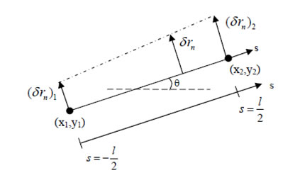
As shown in the diagram above, l is the length of an element represented by a straight line, s is a local coordinate along
this element and θ is the angle of node 2 measured from the horizontal with respect to node 1. The positions of the two
nodes, (x1, y1) and
(x2, y2) fully specify the geometry of the
element. Using l and θ,
we can relate to the nodal positions
as l cosθ = x2-x1 and
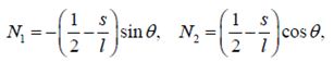
l sinθ = y2-y1. The virtual motion of the interface relates to the virtual motion of the nodal positions
by a straight line interpolation. This is given by:
![]()
where,
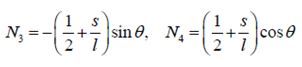
Similarly, the interface velocity relates to the nodal velocities
as follows:
![]()
Forces acting on the nodes
The surface tension depends on the crystalline orientation
of the interface which can be described by a function γ (θ).
For an interface modeled by straight line elements, γ (θ) is
constant on each element, but takes different values on
elements of different slopes. For a two dimensional structure,
the total free energy is given by:
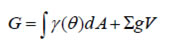
The first part of summation is over the lengths of all the
elements, and the second over areas of all the phases.
For the virtual motion of single element, the total free
energy G varies as:
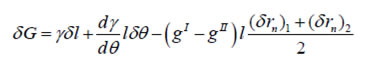
The first term is due to the elongation of the element: the
second due to the rotation and the third due to the trapezoidal
area swept by the motion, where gI and gII are the free energy densities of the two bulk phases. Here we can express the free energy variation in terms of virtual motion of the nodes.
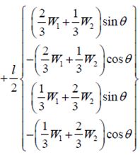
![]()
Here fi are the forces acting on the nodes and resolving the
forces along the x and y directions, we obtain:
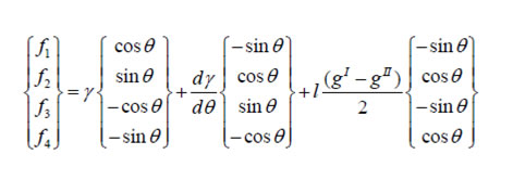
The force vector includes physical effects such as elastic or electrostatic energy. However, we neglect W and ![]() for our simulations.
for our simulations.
Implementing the Finite Element Method
The mobility L also depends on the crystalline direction of the interface. For an interface modeled by straight line elements,
L is constant on each element, but can take different values on elements of different slopes. We can write the weak statement
as follows:
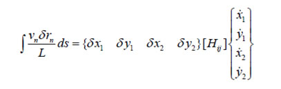
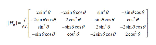
where [Hij] is a 4 x 4 symmetric matrix calculated from
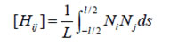
which gives:
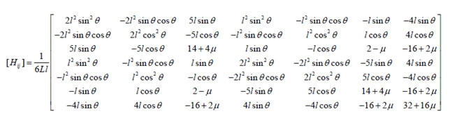
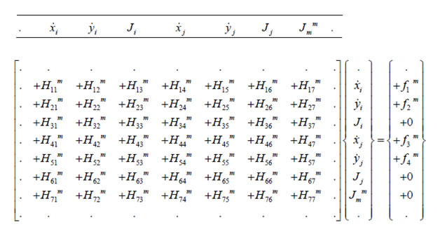
For our simulation, we have 7 x 7 H matrix instead of 4 x 4 H
matrix as shown below.
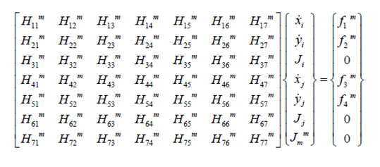
Assemble contributions from all elements
We can first construct a global H matrix with all zero elements.
Then count all the elements, calculate each 7 x 7 local H matrix
and add them to the correct locations in the global H matrix. An example to add element m to the global matrix is shown below.
Determining the instant two particles meet
We measured the angles of the node of the first particle with respect to all the other nodes of the second particle in order to determine the instant in which two particles meet.
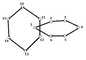
The diagram above shows the schematic when one node
of particle is inside the other particle. We measured the angle between node 1 and the nodes 10 - 15. the angle is always
measured with respect to the horizontal as shown below:
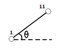
Adding up all these angles, if the sum of the angles is = (360 ± 2)° ,
it means the node is inside the second particle. When this
happens we proceed to remove the corresponding elements
and node as shown in the schematic diagram below. The red
lines represents the nodes and elements to be removed while
the dotted lines represents the new elements. One thing to
note is that the labelling of the nodes on both the particles
must be in a clockwise direction to facilitate the re-combining
of the nodes.
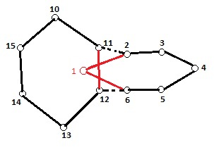
We then created the new force and H matrix with the new coordinates of the combines particles and calculated the new velocities.