Chapter
4
Geometric
Representations
for Arbitrary Hierarchies
In the last chapter, we saw the complex
mechanics of classical central place theory come alive as a single
dynamic
system when viewed through the lens of fractal geometry. The fit
of the classical and fractal geometric hierarchies is exact.
Thus,
as one might use a carefully surveyed topographic map, with
field-checked
spot elevations, as a guide into dense jungle or other unsurveyed
landscapes,
so too we use our carefully field checked alignment of the classical
and
the fractal as a guide into unseen or unproven areas of theoretical
geography.
The difference is that the "field" tests in one case occur in
"terrestrial
space" while in the other the "field" tests occur in "geometry, number
theory, and pure mathematics."
We saw hexagonal hierarchies, of
different
orientation, cell size, and stacking characteristics, arise from the
same
base of unit hexagons. These were associated with three
integers:
3, 4, and 7. The thoughtful reader might naturally ask a number
of
questions, such as:
- are there other numbers that would
serve as K
values or are 3, 4, and 7 the only such values?
- are 5 or 6 possible K
values?
- are there K values
larger
than 7?
- how many K values are
there?
Dacey
considered these issues. - How
does one determine the number of
sides
in a fractal generator that will generate a correct hierarchy for
arbitrary K
values?
- How does one determine fractal
generator shape
that will generate a correct hierarchy for arbitrary K values?
In this chapter we offer geometric
representations
for higher numerical K values. Subsequent chapters will
develop
the number theory required to execute these constructions.
Coordinatization
of
the triangular lattice
Previous
chapters employed a lattice of points to represent central places as a
synthetic (coordinate-free) system. It is straightforward to
assign
a coordinate system, as well. If a point is given the usual
Euclidean
coordinate (x,y), based on perpendicular axes, its distance from
the origin is easily calculated to be (x2 + y2)1/2.
Thus, there is a natural association of the quadratic expression x2
+ y2 with the point (x,y). Such
an
expression is sometimes called a quadratic form. Quadratic forms
have been studied extensively and material about them will appear in
Chapter
5.
When the plane is
occupied by a set of hamlets, each equidistant from its nearest
neighbors,
it seems more reasonable to pick a coordinate system which gives
coordinates
(0,0), (1,0), and (0,1) to three hamlets which are vertices of an
equilateral
triangle. Thus it is natural to have a horizontal
x-axis and
a y-axis at angle 60° to the x-axis, as illustrated in
Figure 4.1. Now, however, the calculation of distance between a
point
with coordinates (x,y) and the origin (0,0) is more
complicated.
Figure 4.1 illustrates the situation when x and y are
both
positive. The right triangle whose hypotenuse has length this
distance
now has vertical side of length  y/2
and horizontal side of length y/2+x. Thus the
distance,
d,
is
y/2
and horizontal side of length y/2+x. Thus the
distance,
d,
is

The quadratic form
x2
+
xy
+ y2 is thus associated with the vertex
(x,y)
as both Dacey and Loeb
had suggested earlier.Figure 4.1.
The standard y-axis of Cartesian coordinates is shown in cyan
(turquoise).
The yellow lines show the oblique axes. The value d
represents
the distance between the origin and an arbitrary point, (x,y),
drawn in this case on the line y = x of the oblique
axes.
The illustration in Figure 4.1 shows
both values as positive. Thus, it must be established that this
distance
is the same even when
x and
y are not both positive.
When
x and y are both negative. |x| must be
substituted for x, and |y| must be substituted for y,
but the calculation remains the same.
When exactly one
of x or y becomes negative, the geometry is
different.
Now the vertical side of the relevant right triangle has side of length
|y|/2
but the horizontal side is now of length
x-|y|/2.
Thus the appropriate distance is
When x
is negative and y is positive, a
similar
calculation results.
Thus the form x2
+
xy
+ y2 is indeed associated with the vertex
(x,y)
in this coordinate system. Any positive integer that is equal to
x2
+
xy
+ y2 for some integers x
and y is called
Löschian,
after August Lösch.
One mathematical question that then occurs is: what integers are
Löschian? The next chapter (Chapter 5) develops the number theory
necessary to answer that question. Other issues involve values of
K
greater than 7 as well as questions involving number of generator sides
and generator shape mentioned above. The rest of this chapter
deals
with these items.
Higher K-values:
An Infinite Number
Earlier research, by
August Lösch, Michael Dacey,
and others shows illustrations of K-values greater than
7.
Indeed, research by Arthur Loeb,
in crystallography, and Dacey,
in
geography, led to independent discovery that the Diophantine
equation, x2+xy+y2 = K
would generate all K values when pairs of positive integers
were
substituted for x and for y. Thus, when (x,y)=(1,1)
the equation x2+xy+y2 = K
yields
a value of K=3; when (x,y)=(0,2), it follows that
K=4;
and, when (x,y)=(1,2), it follows that K=7.
Pairs such as (0,0) and (1,0) yield only trivial results so that the
values
of 3, 4, and 7 are the three smallest K-values. There are
no other K values less than 7.
The result of Loeb/Dacey is important
because
it shows
- that there is an infinite number
of
possible K
values
- that this infinity of values is in
one-to-one
correspondence with the integral lattice points in the plane
- that one can give a numerical
generating function
to create K values
Thus, a graph of lattice points in the
plane
offers a convenient method of visualizing K-values larger than
7
(Figure 4.2).
 Figure 4.2.
The coordinatized lattice points in yellow transform into K-values
in cyan using the Diophantine equation K=x2+xy+y2
Figure 4.2.
The coordinatized lattice points in yellow transform into K-values
in cyan using the Diophantine equation K=x2+xy+y2 |
The
Diophantine
equation, x2+xy+y2 = K,
is
symmetric: the points (1,2) and (2,1) represent different
locations
in the plane. They both generate the same K value.
Thus,
it suffices to consider only a portion of the available lattice
points:
those in the first quadrant on one side of the line y=x. Because
the pattern of points associated with central place hierarchies is
based
on a triangular lattice, the graph of lattice points displayed in
Figure
4.2 is based on an oblique, rather than on a rectangular, coordinate
system
with angles at the origin of 60 and 120 degrees. Combining
considerations
of symmetry and oblique coordinates led to Figure 4.2. In that
figure,
both coordinate pairs, and corresponding K-value generated by
the
Diophantine equation, are shown.
With an
infinite
number of K-values available, it is a daunting consideration to
try to figure out how to create a nested hierarchy of hexagonal trade
areas
suited to each value of K. Simple drawing skills do not
suffice.
One needs a formal strategy that can be replicated at will.
Fractal
geometry will offer that capability.
In the previous chapter, fractal
generators
appear simply to be plucked out of thin air: there is art in
generator
selection. Actually, the generator for the K=7 hierarchy
suggested
itself naturally with observations of overfit/underfit of the six small
hexagons in relation to the boundary of the next larger one (Figure
4.3).
From there, it was simply a matter of educated guessing and trial and
error
to find generators for K=3 and K=4 hierarchies.
Someone
with considerable experience working with this approach might, for
example,
figure out a fractal generator for a K=76 hierarchy, associated
with the lattice point (4,6) (Figure 4.4). For replication by
arbitrary
individuals to be successful, however, one needs to capture the art in
the formalized theory and language of mathematics: to transform
art
into science.

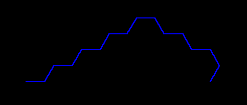
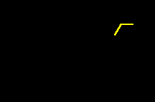
Figure
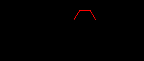
4.3.
Overfit and underfit of small to larger hexagons emphasized:
fractal
generator, a zig-zag three sided shape, emerges from such observation.
|
Figure 4.4.
K=76
fractal generation; corresponding lattice point has coordinates
(4,6).
The generator shape appears at the edge. |
Fractal
Generation
of Arbitrary K-Values: Geometric Evidence
Once one
generator
shape is known, can it be used to determine other generator
shapes?
The answer is yes. The table in Table 4.1 illustrates that the K=3
generator, with a half a "hexstep" added, leads to the K=7
generator.
| K=3
generator. |
 |
| K=3
generator
(red) with one half hexstep added (green). |
 |
| K=7
generator |
 |
Table 4.1. The K=3
generator
leads to the K=7 generator.
To try to
uncover
pattern useful in creating fractal generators for arbitrary K
values,
we begin by looking at a subset of K values: those along
the
y-axis,
only. In that case, because
x2+xy+y2
= 0 + 0 + y2 = K , it follows that
the square
root of K is an integer and that the lattice points (0,y)
on the y-axis may be rewritten as (0,  ).
Trial and error with finding fractal generators for selected values
along
the y-axis produced the table of generators shown in Figure
4.5.
The trivial value of K=1, associated with the point (0,1) is
not
shown in this figure. Within that "trial and error" process a
pattern
emerged, demonstrated in the animated Figure 4.5.
).
Trial and error with finding fractal generators for selected values
along
the y-axis produced the table of generators shown in Figure
4.5.
The trivial value of K=1, associated with the point (0,1) is
not
shown in this figure. Within that "trial and error" process a
pattern
emerged, demonstrated in the animated Figure 4.5.
- Begin with the K=4
generator
(lowest
value on the y-axis): generator in red.
- To the previous generator, add a
full hexstep
to the left of it and a half hexstep, curled under, to the right:
generator in green. This new generator produces the K=9
hierarchy.
- To the previous generator, add a
half hexstep
to the left (flat portion of the step): generator in blue.
This new generator produces the K=16 hierarchy.
- Add two full hexsteps, one on each
side, to
the K=4 generator, creating a symmetric generator that produces
the K=25 hierarchy.
- To the previous generator, add a
full hexstep
to the left of it and a half hexstep, curled under, to the right:
generator in green. This new generator produces the K=36
hierarchy.
- To the previous generator, add a
half hexstep
to the left (flat portion of the step): generator in blue.
This new generator produces the K=49 hierarchy.
- Add two full hexsteps, one on each
side, to
the K=25 generator, creating a symmetric generator that
produces
the K=64 hierarchy.
- To the previous generator, add a
full hexstep
to the left of it and a half hexstep, curled under, to the right:
generator in green. This new generator produces the K=81
hierarchy.
- To the previous generator, add a
half hexstep
to the left (flat portion of the step): generator in blue.
This new generator produces the K=100 hierarchy.
| Lattice Coordinate |
K-value (y-axis values) |
Generator Shape |
Hierarchy Type |
| (0,2) |
K=4 |

|
4 |
| (0,3) |
K=9 |

|
3 |
| (0,4) |
K=16 |

|
7 |
| (0,5) |
K=25 |

|
4 |
| (0,6) |
K=36 |

|
3 |
| (0,7) |
K=49 |
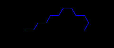
|
7 |
| (0,8) |
K=64 |
|
4 |
| (0,9) |
K=81 |

|
3 |
| (0,10) |
K=100 |
|
7 |
Figure 4.5. Fractal
generators
for selected values on the
y-axis of lattice points generated by
x2+xy+y2
= K. Animation and static versions.
Broadly speaking, we observe the
following
pattern (refer for this discussion to the static portion of Figure 4.5;
the colors match).
- (0,2), K=4.
Begin with the isosceles trapezoidal shape of the K=4 hierarchy.
- Note its bilateral symmetry
about a
vertical
line.
- Note that it takes two sides to
climb the
right side to the top of the generator
- (0,3), K=9.
For K=9, begin with the K=4 generator and
- add one full hex-step to the left
- add one half hex-step to the
right,
tucked
under at 120 degrees
- note that it takes three sides
to
climb the
right side to the top of the generator, one more than it did for the
"begin"
value
- (0,4), K=16.
For K=16, begin with the K=9 generator and
- add one half level part of a
hex-step to the
left
- note that it takes the same
number
of sides
to climb the right side to the top of the generator as it did in the
previous
case.
- (0,5), K=25.
For K=25, begin with the K=4 generator and
- add a full hex-step to the left
- add a full hex-step to the right
- note that it takes four sides to
climb the
right side to the top of the generator
- note the bilateral symmetry
about a
vertical
line
- (0,6), K=36.
For K=36, begin with the K=25 generator and
- add one full hex-step to the left
- add one half hex-step to the
right,
tucked
under at 120 degrees
- note that it takes one more side
to
climb
the right side to the top of the generator than it did for the "begin"
value
- (0,7), K=49.
For K=49, begin with the K=36 generator and
- add one half level part of a
hex-step to the
left
- note that it takes the same
number
of sides
to climb the right side to the top of the generator as it did in the
previous
case.
- (0,8), K=64.
For K=64, begin with the K=25 generator and
- add a full hex-step to the left
- add a full hex-step to the right
- note that it takes six sides to
climb the
right side to the top of the generator
- note the bilateral symmetry
about a
vertical
line
- (0,9), K=81.
For K=81, begin with the K=64 generator and
- add one full hex-step to the left
- add one half hex-step to the
right,
tucked
under at 120 degrees
- note that it takes one more side
to
climb
the right side to the top of the generator than it did for the "begin"
value
- (0,10), K=100.
For K=100, begin with the K=81 generator and
- add one half level part of a
hex-step to the
left
- note that it takes the same
number
of sides
to climb the right side to the top of the generator as it did in the
previous
case.
.........continue,
using the pattern without Figure 4.5.........
- (0,11), K=121.
For K=121, begin with the K=64 generator and
- add a full hex-step to the left
- add a full hex-step to the right
- note that it takes eight sides
to
climb the
right side to the top of the generator
- note the bilateral symmetry
about a
vertical
line
- (0,12), K=144.
For K=144, begin with the K=121 generator and
- add one full hex-step to the left
- add one half hex-step to the
right,
tucked
under at 120 degrees
- note that it takes one more side
to
climb
the right side to the top of the generator than it did for the "begin"
value
...............
After a number of
cases, there appears to be a clear pattern, color-coded as
red-green-blue.
If that pattern is correct, then the reader could, through successive
(but
perhaps tedious) application of this pattern, produce a fractal
generator
for an arbitrary value on the y-axis. We will show a more
systematic
procedure later in this Chapter for finding generator size and shape;
it
will, however, be based on the observations above, so it is important
that
the reader have a clear understanding of them.
To produce
generators
for K-values not on the y-axis is also a simple matter of examining
pattern.
Figure 4.6 shows how to form generators for all other K-values
(not
on the y-axis) simply by adding hex-steps to the y-axis
K-value
generators as one moves to the right across lines of lattice points
parallel
to the line
y=x (cyan lines in Figure 4.7).
Thus, the reader could then form a fractal generator for an arbitrary K-value.
| Y-axis value and line
position |
Fractal generators off the y-axis
as determined by y-axis generator shape. |
| (0,0):
the
first generator appears for K=3 (not on the y-axis; K=0,
on the y-axis, is disregarded) and subsequent generators appear
for K-values of 12, 27, and 48 as one moves to the right across
the line y=x. |
 |
| (0,1):
the
first generator appears for K=7 (not on the y-axis; K=1,
on the y-axis, is disregarded) and subsequent generators appear
for K-values of 19, 37, and 61 as one moves to the right across
the line displaced by 1 from, and parallel to, the line y=x. |
 |
| (0,2):
the
first generator appears for K=4 and subsequent generators
appear
for K-values of 13, 28, 49, and 76 as one moves to the right
across
the line displaced by 2 from, and parallel to, the line y=x. |
 |
| (0,3):
the
first generator appears for K=9 and subsequent generators
appear
for K-values of 21, 39, 63, and 93 as one moves to the right
across
the line displaced by 3 from, and parallel to, the line y=x. |
 |
Figure 4.6.
Fractal
generators are produced for arbitrary
K-values from y-axis
K-values.
See the cyan lines in Figure 4.7.
Fractal
Generation
of Arbitrary K-Values: the Cross-cut Equation as
a Systematic Characterization of Generator Size and Shape
In Figure 4.5, the
"red" category corresponds to a generator type similar to the K=4
generator: an isosceles trapezoid with some number of hex-steps
on
either side, producing a bilaterally symmetric form. The "blue"
category
corresponds to a generator type similar to the K=7 category,
identical
to the previous case but with one half level hex-step added to the
left.
If one looks at the trivial cases of K=0 and K=1 in
Figure
4.6, this style of pattern is evident in moving from K=3 to K=7.
Thus, it appears that there are really only three basic, or primitive,
styles of generator type: K=3 (green), K=4 (red), and K=7
(blue). Because generator shape on the y-axis determines
generator
shape off the axis along rays parallel to the line y=x (cyan
lines in Figure 4.7), we next consider partitioning the set of all K
values according to these three categories using a set of parallel rays
(cyan lines in Figure 4.7) to create that partition. Thus, we
seek
another equation to represent that partition with the intent of using
it
to cut across the Diophantine equation and provide straightforward
solution
to finding the number of sides and the shape of fractal generators for
arbitrary K-values.
The
pattern of numerical K values along rays parallel to y=x,
shown as cyan lines, is captured in Figure 4.7. Thus,
- along y=x,
we have K=3x2 : the K values
along
that ray, only, are generated exactly by substituting 0, 1, 2, 3, 4,...
into that equation yielding K values of 0, 3, 12, 27, 48, ...
- along the
ray
displaced
1 unit from the line y=x, we have K=3x2+3x+1:
the K values along that ray, only, are generated exactly by
substituting
0, 1, 2, 3, 4,... into that equation yielding K values of
1, 7, 19, 37, 61,...
- along the
ray
displaced
2 units from the line y=x, we have K=3x2+6x+4:
the K values along that ray, only, are generated exactly by
substituting
1, 2, 3, 4,... into that equation yielding K values of 4, 13, 28, 49,
76,...
- along the
ray
displaced
3 unit from the line y=x, we have K=3x2+9x+9:
the K values along that ray, only, are generated exactly by
substituting
0, 1, 2, 3, 4,... into that equation yielding K values of 9,
21,
39, 63, 93,...
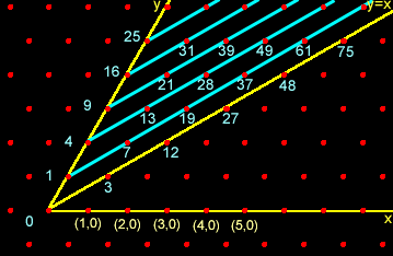
Equations for
y=x
and cyan rays parallel to y=x:
- K=3x2
for
the line y=x
- K=3x2
+
3x +1, for the cyan line displaced by 1
- K=3x2
+
6x +4, for the cyan line displaced by 2
- K=3x2
+
9x +9, for the cyan line displaced by 3
|
Figure 4.7.
Pattern suggesting cross-cut equation. The equation for the cyan
rays, parallel to y=x, generate exactly the K-values
associated with lattice points along that ray (when integers are
substituted
into those equations..
Generalizing from
the observed pattern, it appears that the equation K=3x2
+
3bx +b2, where b counts the number of
units
the ray is displaced from y=x, will serve to capture all
the K-values associated with the lattice points along a single
horizontal
ray parallel to y=x (cyan, Figure 4.7), and to capture
no
others elsewhere. This idea is stated in the following theorem;
the
next chapter will present some of the number theoretic infrastructure
behind
it.
Fundamental
Theorem (S. Arlinghaus, 1985,
and
S. Arlinghaus in S. and W. Arlinghaus, 1989).
In a
triangular
central place lattice, the central place K-values, lying along
any
single one of the rays parallel to the line y=x, are
generated
by substituting non-negative integral values into a quadratic equation K=3x2
+
3bx +b2=3x2+3()x+()2,
where b=0, 1, ..., n,... counts the number of units the
ray
is
translated from y=x.
Thus, any single K
value has two quadratic equations that represent it. We now
proceed
to use properties of these quadratic equations to extract information
from
them sufficient to determine the number of fractal generator sides and
number of hex-steps for arbitrary K values from algebraic
information,
alone. Thus, an informed reader will have the capability to
replicate
the results, independent of relative position on any image. As an
analogy, this process is similar to using latitude and longitude as
numerical
measures to determine absolute position on the earth-sphere rather than
using parallels and meridians as geometric measures to determine
relative
position on the earth-sphere.
Number
of Generator Sides
The patterns observed appear often to involve partitions related to the
number 3. Thus, we consider a value based on divisibility by 3 as
one index.
Define an
integral
value j, using K-values along the y-axis, only,
as:
- If K
is congruent
to 0(mod 3), then j=()
/ 3;
- If K
is
not congruent
to 0(mod 3), then j=(()-1)/3
or j=(()-2)/3,
which
ever is an integer (clearly, both cannot be integers--K leaves
either
a remainder of 1 or of 2 when divided by 3).
As some examples:
- when K=4,
then 4 is not evenly divisible by 3 so that K is not congruent
to
0(mod 3). Thus, one of j=(()-1)/3
or j=(()-2)/3
is
an integer. Indeed, j=(()-2)/3
= (2-2)/3=0 is an integer.
- when K=9, then
9 is evenly divisible by 3 so that K is congruent to 0(mod
3).
Thus, j=() /
3 =
3/3 = 1.
- when K
= 16,
then 16 is not evenly divisible by 3 so that K is not congruent
to 0(mod 3). Thus, one of j=(()-1)/3
or j=(()-2)/3
is
an integer. Indeed, j=(()-1)/3
= (4-1)/3=1 is an integer.
- when K=25,
then 25 is not evenly divisible by 3 so that K is not congruent
to 0(mod 3). Thus, one of j=(()-1)/3
or j=(()-2)/3
is
an integer. Indeed, j=(()-2)/3
= (5-2)/3=1 is an integer.
- when K=36,
then 36 is evenly divisible by 3 so that K is congruent to
0(mod
3). Thus, j=()
/ 3 = 6/3 = 2.
- when K=49,
then 49 is not evenly divisible by 3 so that K is not congruent
to 0(mod 3). Thus, one of j=(()-1)/3
or j=(()-2)/3
is
an integer. Indeed, j=(()-1)/3
= (7-1)/3=2 is an integer.
- when K=64,
then 64 is not evenly divisible by 3 so that K is not congruent
to 0(mod 3). Thus, one of j=(()-1)/3
or j=(()-2)/3
is
an integer. Indeed, j=(()-2)/3
= (8-2)/3=2 is an integer.
- when K=81,
then 8 is evenly divisible by 3 so that K is congruent to 0(mod
3). Thus, j=()
/ 3 = 9/3 = 3.
- when K=100,
then 100 is not evenly divisible by 3 so that K is not
congruent
to 0(mod 3). Thus, one of j=(()-1)/3
or j=(()-2)/3
is
an integer. Indeed, j=(()-1)/3
= (10-1)/3=3 is an integer.
- when K=121,
then 121 is not evenly divisible by 3 so that K is not
congruent
to 0(mod 3). Thus, one of j=(()-1)/3
or j=(()-2)/3
is
an integer. Indeed, j=(()-2)/3
= (11-2)/3=3 is an integer.
- when K=144,
then 144 is evenly divisible by 3 so that K is congruent to
0(mod
3). Thus, j=()
/ 3 = 12/3 = 4.
...............
The examples
above
are color-coded using the scheme of the geometric table to suggest
pattern
in the output of j-values. What the pattern suggests is,
for
K-values
on the y-axis only,
- when K
is congruent
to 0(mod 3), then the number of sides for a fractal generator is given
by 2+4j
- when K
is not
congruent to 0(mod 3), then the number of sides for a fractal generator
is given by 3+4j.
Number
of Generator Hex-steps: Generator Shape
To count the number of hex-steps for an arbitrary K-value on
the
y-axis, we employ not only the j-value calculated in the
previous
section, but also the well-known discriminant (square root of (B2
-
4AC) in Ax2 + Bx + C) of a quadratic
form. Once again, we begin by considering a number of
examples
in order to study pattern and to piece it together with other pattern
that
is known. From the Fundamental Theorem, we know that
K=3x2+3()x+()2.
The discriminant of this equation is D = (3())2
-
4·3()2= 9K
- 12K = -3K. To count the number of hex-steps for a
fractal
generator for a y-axis
K-value, follow the strategy below:
- if K
is
congruent
to 0(mod 3) and
- if D
is congruent
to 1(mod 4), then the number of generator hex-steps is equal to the
greatest
integer in (2+4j)/2 =1+2j.
- if D
is congruent
to 0(mod 4), then the number of generator hex-steps is equal to the
greatest
integer in (2+4j)/2=1+2j.
- if K
is
not congruent
to 0(mod 3) and
- if j
is
even
(divisible by 2) then
- if D
is congruent
to 1(mod 4), then the number of generator hex-steps is equal to the
greatest
integer in (3+4j)/2.
- if D
is congruent
to 0(mod 4), then the number of generator hex-steps is equal to the
greatest
integer in (5+4j)/2.
- if j is
odd (not
divisible by 2) then
- if D
is congruent
to 1(mod 4), then the number of generator hex-steps is equal to the
greatest
integer in (5+4j)/2.
- if D
is congruent
to 0(mod 4), then the number of generator hex-steps is equal to the
greatest
integer in (3+4j)/2.
Looking at some
examples,
again, the color-coding of red-green-blue shows that the number
theoretic
patterns provide an exact fit with the geometric pattern and they do so
without requiring seeing previous cases: the number theoretic
patterns
offer absolute measures, replicable independent of examination of
previous
cases.
Thus, for K-values
on the y-axis,
- when K=4,
then D = -3K = -12 which is evenly divisible by
4.
In addition, K is not congruent to 0(mod 3) and j=0
from
above, which is even. Thus, the number of hex-steps is the
greatest
integer in (5+4j)/2 which is 2.
- when K=9, then D
= -3K = -27 which is not evenly divisible by 4 and leaves a
remainder
of 1. In addition, K is congruent to 0(mod 3) and
j=1 from above. Thus, the number of hex-steps is the greatest
integer in 1+2j which is 3.
- when K
= 16,
then D = -3K = -48 which is evenly divisible by 4.
In addition, K is not congruent to 0(mod 3) and j=1 from
above, which is odd. Thus, the number of hex-steps is the
greatest
integer in (3+4j)/2 which is 3.
- when K=25,
then D = -3K = -75 which is not evenly divisible by 4
and
leaves a remainder of 1. In addition, K is not congruent
to
0(mod 3) and j=1 from above, which is odd. Thus, the
number
of hex-steps is the greatest integer in (5+4j)/2 which is 4.
- when K=36,
then D = -3K = -108 which is not evenly divisible by 4
and
leaves a remainder of 1. In addition, K is congruent
to 0(mod 3) and j=2 from above. Thus, the number of
hex-steps
is the greatest integer in 1+2j which is 5.
- when K=49,
then D = -3K = -147 which is not evenly divisible by
4.
In addition, K is not congruent to 0(mod 3) and j=2
from
above, which is even. Thus, the number of hex-steps is the
greatest
integer in (3+4j)/2 which is 5.
- when K=64,
then D = -3K = -192 which is evenly divisible by
4.
In addition, K is not congruent to 0(mod 3) and j=2 from
above, which is even. Thus, the number of hex-steps is the
greatest
integer in (5+4j)/2 which is 6.
- when K=81,
then D = -3K = -243 which is not evenly divisible by 4
and
leaves a remainder of 1. In addition, K is
congruent
to 0(mod 3) and j=3 from above. Thus, the number of
hex-steps
is the greatest integer in 1+2j which is 7.
- when K=100,
then D = -3K = -300 which is evenly divisible by
4.
In addition, K is not congruent to 0(mod 3) and j=3 from
above, which is odd. Thus, the number of hex-steps is the
greatest
integer in (3+4j)/2 which is 7.
- when K=121,
then D = -3K = -363 which is not evenly divisible by 4
and
leaves a remainder of 1. In addition, K is not congruent
to
0(mod 3) and j=3 from above, which is odd. Thus, the
number
of hex-steps is the greatest integer in (5+4j)/2 which is 8.
- when K=144,
then D = -3K = -432 which is not evenly divisible by 4
and
leaves a remainder of 1. In addition, K is
congruent
to 0(mod 3) and j=4 from above. Thus, the number of
hex-steps
is the greatest integer in 1+2j which is 9.
...............
Use
of the Fundamental Theorem
The
following
example shows how to determine the b-value corresponding to an
arbitrary
Löschian number and therefore create a second Diophantine expression
of that number. Suppose it has been determined, using the
sufficient
condition given in the Fundamental Theorem, that the number 397 is a
Löschian
number. Express 397 as 3x2 + 3bx +b2,
for some
b. To do so, consider values of b from 0 to
3971/2. The greatest integer in this square root is
19.
Thus, possibilities for b range from 0 to 19. Because 3x2
+ 3bx=397-b2, it follows that 397-b2
must be divisible by 3. This fact eliminates from further
consideration,
as b, any integer between 0 and 19 for which 397-b2
is
not a multiple of 3. These values are shown in the central column
of Table 4.2. Additionally, the material associated with the
Fundamental
Theorem states that the discriminant of the quadratic form, 3x2
+ 3bx +b2 must be an integer. Thus, in
the
right-hand column of Table 4.2 we calculate these discriminants for
each
of the candidate b-values singled out in the central
column.
The only candidate b value that remains is b=1 and
therefore
the correct quadratic form to also associate with 397 is 3x2
+ 3x +1. Geometrically, the ordered pair that generates
397
is represented as a lattice point that lies along the line b=1,
displaced one unit from the line y=x in the oblique
coordinate
system.
| b |
(397-b2)/3 |
Square root of discriminant |
| 0 |
132.333 |
a |
| 1 |
132 |
47611/2=69 |
| 2 |
131 |
47521/2=68.934 |
| 3 |
129.333 |
a |
| 4 |
127 |
47161/2=68.673 |
| 5 |
124 |
46891/2=68.476 |
| 6 |
120.333 |
a |
| 7 |
116 |
46171/2=67.948 |
| 8 |
111 |
45721/2=67.616 |
| 9 |
105.333 |
a |
| 10 |
99 |
44641/2=66.813 |
| 11 |
92 |
44011/2=66.340 |
| 12 |
84.333 |
a |
| 13 |
76 |
42571/2=65.245 |
| 14 |
67 |
41761/2=64.621 |
| 15 |
57.333 |
a |
| 16 |
47 |
39961/2=63.213 |
| 17 |
36 |
38971/2=62.425 |
| 18 |
24.333 |
a |
| 19 |
12 |
36811/2=60.671 |
Table 4.2.
This table shows candidate values for b for K=397 in
the
left-hand column. It shows values of (397-b2)/3
for each of those candidate values in the center column. The
right-hand
column shows the square root of the discriminant of the quadratic
expression
3x2 + 3bx +b2 for different
values of b (from 0 to 19) that produce an integral value in
the
center column.
Now we have two
quadratic
equations to solve simultaneously to obtain the ordered pair that gives
rise to the Löschian value of 397.
397 = 3x2
+ 3x + 1
397 = x2
+ xy + y2
Solving the first
equation
using standard techniques from high school algebra, and choosing the
positive
value, gives x = 11. Use that value of x to find y
= 12 in the second equation. There are no other
lattice
points that give rise to this particular Löschian number because there
is no other integral discriminant of the quadratic form 3x2
+ 3bx +b2.
The geometric characterization of the central place lattice as a set of
integral lattice points lying along a set of lines parallel to y
= x resulted, after some work, in a Fundamental Theorem that
permits
the algebraic determination of a quadratic form, 3x2
+ 3bx +b2 , to generate a set of lattice
points
lying along a single line. When this second quadratic form was
applied
to the Diophantine equation,
K=
x2 + xy
+ y2 , easy calculations permit the determination of
the lattice coordinates associated with an arbitrary Löschian number
and of whether or not those coordinates are unique.
Uniqueness of Löschian
numbers:
solutions to previously unsolved problems.
Solving
the K-value Twin Hierarchy Problem
Dacey
noticed that some K-values have more than one central place
hierarchy
associated with them. Using classical methods, however, it is
difficult
to determine what these hierarchies might look like. Indeed,
Dacey
noted this issue as an unsolved problem in the classical geometry of
central
place theory. The fractal approach, when extended to arbitrary K-values,
permits solution of this unsolved problem using the Fundamental Theorem
and associated constructions.
Suppose
it has been determined that the number 49 is a Löschian number.
Express 49 as 3x2 + 3bx +b2,
for some
b. To do so, consider values of b from 0 to
491/2. The greatest integer in this square root is
7.
Thus, possibilities for b range from 0 to 7. Because 3x2
+ 3bx=49-b2, it follows that 49-b2
must be divisible by 3. This fact eliminates from further
consideration,
as b, any integer between 0 and 7 for which 49-b2
is
not a multiple of 3. These values are shown in the central column
of Table 4.3. Additionally, the material associated with the
Fundamental
Theorem states that the discriminant of the quadratic form, 3x2
+ 3bx +b2 must be an integer. Thus, in
the
right-hand column of Table 4.3 we calculate these discriminants for
each
of the candidate b-values singled out in the central
column.
The only candidate b values that remains are b=2 and b=7
and therefore the correct quadratic forms to also associate with 49 are
3x2 + 6x + 4 and 3x2 + 21x
+49.
Geometrically, the ordered pairs that generate 49 are represented as a
lattice points that lies along the line b=2, displaced two units
from the line y=x in the oblique coordinate system, and
along
the line b=7, displaced seven units from the line y=x
in the oblique coordinate system.
| b |
(49-b2)/3 |
Square root of discriminant |
| 0 |
16.333 |
a |
| 1 |
16 |
5851/2=24.186 |
| 2 |
15 |
5761/2=24 |
| 3 |
13.333 |
a |
| 4 |
11 |
5401/2=23.237 |
| 5 |
8 |
5121/2=22.627 |
| 6 |
4.333 |
a |
| 7 |
0 |
4411/2=21 |
Table 4.3.
This table shows candidate values for b for K=49 in the
left-hand
column. It shows values of (49-b2)/3 for each
of
those candidate values in the center column. The right-hand
column
shows the square root of the discriminant of the quadratic expression 3x2
+ 3bx +b2 for different values of b
(from
0 to 7) that produce an integral value in the center column.
Now we have two
sets
of two quadratic equations each to solve simultaneously to obtain the
ordered
pairs that gives rise to two different hexagonal hierarchies associated
with the Löschian value of 49.
49 = 3x2
+ 6x + 4
49 = x2
+ xy + y2
49 = 3x2
+ 21x + 49
49 = x2
+ xy + y2
In the first
set of equations, x=3 and y=5. In the second set,
x=0
and y=7. There are no other lattice points that give rise
to this particular Löschian number because there is no other integral
discriminant, beyond these two, of the quadratic form 3x2
+ 3bx +b2. Thus, K=49 is
produced
either from the lattice point (0,7) on the y-axis or from the
lattice
point (5,3) not on the y-axis. Figure 4.8 illustrates the
two different fractal generators that give rise to the two different
hierarchies
using the procedure based on the Fundamental Theorem in associating
fractal
generators with lattice points.
Figure 4.8.
Geometric
solution of the K=49 twin hierarchy puzzle. The left
frame
shows an 11-sided generator formed from the ordered pair (0,7) on the y-axis,
yielding a K=7 type of hierarchy. The right frame shows a
9-sided generator formed from the ordered pair (5,3), not on the y-axis,
yielding a K=4 type of hierarchy.
This example
illustrates
the fact that the Fundamental Theorem solves, completely, the
previously
unsolved problem involving uniqueness, and its lack, in calculating
hexagonal
hierarchies. The geometric characterization of the central place
lattice as a set of integral lattice points lying along a set of lines
parallel to y = x resulted, after some work, in a
Fundamental
Theorem that permits the algebraic determination of a quadratic form, 3x2
+ 3bx +b2 , to generate a set of lattice
points
lying along a single line. When this second quadratic form was
applied
to the Diophantine equation,
K= x2 + xy
+ y2 , easy calculations permit the determination of
the lattice coordinates associated with an arbitrary Löschian number
and also the determination of whether those coordinates are unique.
Putting
the Pieces Together
The material in the previous sections indicates a plausible strategy
for
producing appropriate fractal generators that will create, through
iteration,
exact central place hierarchies for arbitrary
K-values. It
does so using only number theoretic properties of two quadratic
forms.
Thus, process is replicable and independent of previous cases. In
the next chapter we consider some of the number theoretic
infrastructure
on which these methods rest and in a final chapter we present some real
world considerations.
Institute
of Mathematical Geography. Copyright, 2005, held by authors.
Spatial Synthesis:
Centrality and Hierarchy, Volume I, Book 1.
Sandra Lach Arlinghaus and
William Charles Arlinghaus