Figure 1 shows a numerically approximated partial bifurcation set for
system (1).![]() In region I there is always a stable
Cournot-Nash equilibrium point at which the incumbent has a reelection
advantage (i.e., p>.5). In region II, flows spiral away from the fixed
point, approach a saddle point and then wander into a situation in which not
only does the incumbent have an electoral advantage, but the challenger
receives no contributions. In region III there is a stable limit cycle
(Hirsch and Smale 1974, 250). Flows converge to an indefinitely repeated
oscillation through most but not all of which the incumbent has an advantage.
In region IV there are no stable fixed points. Flows wander rapidly to states
in which p=1. In region V, flows converge to the interior of a homoclinic
cycle
In region I there is always a stable
Cournot-Nash equilibrium point at which the incumbent has a reelection
advantage (i.e., p>.5). In region II, flows spiral away from the fixed
point, approach a saddle point and then wander into a situation in which not
only does the incumbent have an electoral advantage, but the challenger
receives no contributions. In region III there is a stable limit cycle
(Hirsch and Smale 1974, 250). Flows converge to an indefinitely repeated
oscillation through most but not all of which the incumbent has an advantage.
In region IV there are no stable fixed points. Flows wander rapidly to states
in which p=1. In region V, flows converge to the interior of a homoclinic
cycle![]() and then to a stable fixed
point at which p=0. In region VI the incumbent usually ends up getting
virtually no contributions but nonetheless runs at only a slight disadvantage
(.45<p<.5). For h very near zero, however, the flows become highly
irregular and unpredictable. For h=0, a frequent outcome is p=1 and
contributions to the incumbent increasing exponentially with time.
and then to a stable fixed
point at which p=0. In region VI the incumbent usually ends up getting
virtually no contributions but nonetheless runs at only a slight disadvantage
(.45<p<.5). For h very near zero, however, the flows become highly
irregular and unpredictable. For h=0, a frequent outcome is p=1 and
contributions to the incumbent increasing exponentially with time.
***** Figure 1 about here *****
Table 1 shows payoffs to the incumbent and challenger from the
system (1) subgame for several local maximum and
effective boundary pairs (g, h), arrayed so as to define
the strategic form of the first-stage game. A (g, h) pair is a
local maximum if small increases and small decreases in g both produce a
worse payoff for the incumbent, or if small increases and small decreases in
h both produce a worse payoff for the challenger. A (g, h)
pair is an effective boundary if ![]() and the payoffs from system
(1) do not materially change as g becomes more extreme. For
instance, if g decreases below g=-.08 while h=0, the
incumbent's payoff from system (1) remains zero while the challenger
receives the maximum possible payoff,
and the payoffs from system
(1) do not materially change as g becomes more extreme. For
instance, if g decreases below g=-.08 while h=0, the
incumbent's payoff from system (1) remains zero while the challenger
receives the maximum possible payoff, ![]() . Table 1 also
includes the payoffs from all the (g, h) pairs produced by crossing
the g and h values from the local maximum and effective boundary
pairs. The maximum payoffs, denoted
. Table 1 also
includes the payoffs from all the (g, h) pairs produced by crossing
the g and h values from the local maximum and effective boundary
pairs. The maximum payoffs, denoted ![]() and
and ![]() , can
each be arbitrarily large, depending on the length of time the system is
imagined to run before the election. For the runs of about two time units
used to construct Table 1, reasonable valuations are
, can
each be arbitrarily large, depending on the length of time the system is
imagined to run before the election. For the runs of about two time units
used to construct Table 1, reasonable valuations are ![]() .
.
***** Table 1 about here *****
The game of Table 1 does not have a Nash equilibrium in pure
strategies. The mixing probabilities for a mixed-strategy Nash equilibrium
are shown in Table 2.![]() The mixing probabilities imply
that the most likely outcome is the pair
The mixing probabilities imply
that the most likely outcome is the pair ![]() . Using
. Using ![]() gives
gives ![]() ,
, ![]() ,
,
![]() and
and ![]() .
.
***** Tables 2 about here *****
Three of the four outcomes that have positive probability in the mixed-strategy equilibrium imply non-competitive elections. When (g,h)=(-.025, 0), system (1) does not have a stable fixed point. Flows rapidly diverge in such a way that the probability that the incumbent wins the election falls to zero, resulting in a payoff to the incumbent of zero. I interpret this outcome as a case in which the incumbent drops out of the race: only if the incumbent retires is it certain that the incumbent will not win. When (g,h)=(-.025,.487) or (g,h)=(.0425,0), system (1) also lacks a stable fixed point, but in these cases the probability that the challenger wins the election falls to zero. The natural interpretation of these cases is that the incumbent is running unopposed.
Of the four mixed-strategy equilibrium (g,h) pairs, only
![]() induces dynamics that imply probabilities of election
victory that are not either zero or one. A first-stage outcome of
induces dynamics that imply probabilities of election
victory that are not either zero or one. A first-stage outcome of
![]() leads to a competitive campaign in which the
incumbent has a substantial advantage in terms of financial contributions and
chances of reelection. With
leads to a competitive campaign in which the
incumbent has a substantial advantage in terms of financial contributions and
chances of reelection. With ![]() , the point
, the point
![]() is a
fixed point that is a Cournot-Nash equilibrium:
is a
fixed point that is a Cournot-Nash equilibrium: ![]() ,
, ![]() and
and 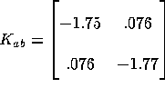 . In qualitative
dynamic terms,
. In qualitative
dynamic terms, ![]() is a center (Hirsch and Smale 1974, 95):
flows in a neighborhood of
is a center (Hirsch and Smale 1974, 95):
flows in a neighborhood of ![]() are attracted to a surface of
closed periodic orbits that surround
are attracted to a surface of
closed periodic orbits that surround ![]() . Figure 2
illustrates the pattern of convergence to the attracting surface and the
magnitude of the variations around the periodic orbits. The figure shows a
flow in system (1) for
. Figure 2
illustrates the pattern of convergence to the attracting surface and the
magnitude of the variations around the periodic orbits. The figure shows a
flow in system (1) for ![]() , beginning
with (r,q,a,b) near
, beginning
with (r,q,a,b) near ![]() . The flow rapidly converges to a
closed orbit.
. The flow rapidly converges to a
closed orbit.![]() Around the closed orbit
the probability that the incumbent wins the election varies between .655 and
.68. Contributions to the incumbent range from .8 to 1.1, while
contributions to the challenger range from .51 to .55.
Around the closed orbit
the probability that the incumbent wins the election varies between .655 and
.68. Contributions to the incumbent range from .8 to 1.1, while
contributions to the challenger range from .51 to .55.
***** Figure 2 about here *****
The (g,h) pair ![]() is a bifurcation point for system
(1): small changes from those values induce qualitative changes in
the system's flows (Guckenheimer and Holmes 1986, 117). Figure 3
magnifies the bifurcation set diagram of Figure 1 near
is a bifurcation point for system
(1): small changes from those values induce qualitative changes in
the system's flows (Guckenheimer and Holmes 1986, 117). Figure 3
magnifies the bifurcation set diagram of Figure 1 near
![]() , which is marked as point O. For (g, h)
values in region III the fixed point is unstable but there is a stable limit
cycle. For (g, h) values in region II the fixed point is a spiral
source and there is at least one saddle point; flows that start near the
source in general approach the saddle point before wandering permanently away
from both fixed points. For (g, h) values in region I the fixed
point is a spiral sink.
, which is marked as point O. For (g, h)
values in region III the fixed point is unstable but there is a stable limit
cycle. For (g, h) values in region II the fixed point is a spiral
source and there is at least one saddle point; flows that start near the
source in general approach the saddle point before wandering permanently away
from both fixed points. For (g, h) values in region I the fixed
point is a spiral sink.![]() Crossing the open segments O-B and O-A, saddle connection
bifurcations occur (Guckenheimer and Holmes 1986, 290-294). Crossing the
open segment O-C, there are Hopf bifurcations (ibid. 1986,
150-152).
Crossing the open segments O-B and O-A, saddle connection
bifurcations occur (Guckenheimer and Holmes 1986, 290-294). Crossing the
open segment O-C, there are Hopf bifurcations (ibid. 1986,
150-152).
***** Figure 3 about here *****
Small variations in the incumbent's choice of a service type g or in the
opposition party's choice of quality h for the challenger may therefore
lead to qualitatively different subgame dynamics. Because the dynamics occur
during a finite time period, the consequences of the qualitative differences
among the dynamics may be in one sense quantitatively small. For
(g,h) values near ![]() , flows that start near the
dynamic equilibrium point
, flows that start near the
dynamic equilibrium point ![]() approach or leave the point so
slowly--after having been quickly attracted to an invariant surface--that in
general at the end of the game the service rate and contributions variables
have values near one of the closed orbits that exist when the equilibrium
values for g and h are chosen exactly. So given similar initial
values for (r,q,a,b), realizations of system (1) that have
different (g,h) values near
approach or leave the point so
slowly--after having been quickly attracted to an invariant surface--that in
general at the end of the game the service rate and contributions variables
have values near one of the closed orbits that exist when the equilibrium
values for g and h are chosen exactly. So given similar initial
values for (r,q,a,b), realizations of system (1) that have
different (g,h) values near ![]() may all leave the
candidates and the contributor in similar quantitative configurations at the
end of the game.
may all leave the
candidates and the contributor in similar quantitative configurations at the
end of the game.