Surface Diffusion and Evaporation-Condensation

To model the diffusion effects on the surface of a nanopartical, we first defined three variables:

j = volume of matter added to the solid surface per unit area and unit time

p = free energy reduction associated with matter per unit volume added the solid t o per unit surface area

m = kinetic parameter in the model

Mass conservation relates the surface velocity to the fluxes of the two matter transport processes.

δi = the volume of matter added to per unit area of the solid surface

δI = mass displacement  

δG = free energy change

The weak statement is:

This is a weak statement including both surface diffusion and evaporation-condensation.  To formulate a method for finite elements, it is convenient to use δI and δr_n as the basic variables.  Eliminating the other variables in the above weak statement, we can rewrite the weak statement as:

Finite Element Method

To approximate a solution of J and v_n, the above weak statement needs to be satisfied for all virtual movements.  However, to implement this process for the finite element method, this requirement can be relaxed such that the weak statement be satisfied for only a family of virtual motions. 

To model the structure, we use a certain number of straight/linear elements connected by nodes.  Each segment is an element, and two neighboring elements meet at a node.  The motions of the nodes constitute the family of virtual motions.  The length of each element can be defined arbitrarily.

In each element, we can define the two nodes based on a Cartesian coordinate system; the two end points of the element, or the two nodes, can be written as (x₁, y₁) and (x₂, y₂).  The element has length, l, and slope θ.  At the mid-point of the element, we can define that midpoint as s.  Due to the surface diffusion process, the two nodal points of the element can move by (δx₁, δy₁) and (δx₂, δy₂).  As a result, we can model the incremental movement by the following equation.

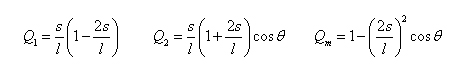
Where the interpolation coefficients can be defined by the following set of equations.

Similarly, the incremental movements of the nodal points can be defined by its corresponding nodal velocities at each direction.

Due to the mass flux vector, we can model the virtual movement of the mass displacement due to diffusion at the nodes to define the δI vector, where,

The interpolation equations can be modeled by a set of quadratic equations atisfying the boundary value problem set forth for each nodal coordinate.

This same interpolation is used for the mass flux J

 From the above relations, we can formulate the element δq^e and vectors, namely,

For each element, the integration gives a bilinear form such that

and the element H^e matrix is

where,

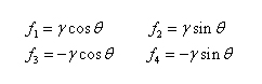
Furthermore, we can specify the driving force due to surface tension acting on each element by the following equations.

With the elemental matrices formed, the finite element process assembles the global H and f matrices such that the global nodal velocities can be computed.  The governing relation in terms of global coordinates can be written as the following

The velocity at each node can then be determined and extracted.

Once the velocity has been extracted, the Euler's method can be utilized to predict the movement of the nodal points.  The Euler's method can then be specified for a user-specified time (and time steps) to model the behavior of the surface diffusion and evaporation process.