Replication Instructions

One of the aims of this book is to encourage others to use similar tools to produce better books and papers. This book has many flaws, some of which come from me not knowing as much as I did when I started the project as I do now, and some of which are just my limitations. I’m sure others can do better. So I’ve tried throughout to be as clear as possible about my methodology, so as to provide an entry point for anyone who wants to set out on a similar project.

This section contains step-by-step instructions for how to build a small-scale model of the kind I’m using. The next chapter discusses the many choice points on the way from small-scale models like this to the large-scale model I use in the book, but it’s helpful to have a small example to start with. I’m going to download the text for issues of the Journal of Philosophy in the 1970s, and build a small (ten-topic) model on them. These instructions assume basic familiarity with R, and especially with tidyverse. If you don’t have that basic familiarity, a good getting-started guide for basic familiarity is Jenny Bryan’s STAT 545: Data wrangling, exploration, and analysis with R, especially chapters 1, 2, 5, 6, 7, 14 and 15. OK, I assume readers are familiar with the basics of R, it’s time to do some basic text mining.

Go to https://jstor.org/dfr and set up a free account.

Download the list of journals JSTOR has. That link will take you to the Excel file; if you’re dedicated to plain text there is also a text version available, but it isn’t a lot of fun to use. The key part of that file is the column title_id. That gives you the code you need to refer to each journal.

Back at https://jstor.org/dfr go to “Create a Dataset” and use “jcode:(jphilosophy)”, or whatever the title_id for your desired journal is, to get a data set.

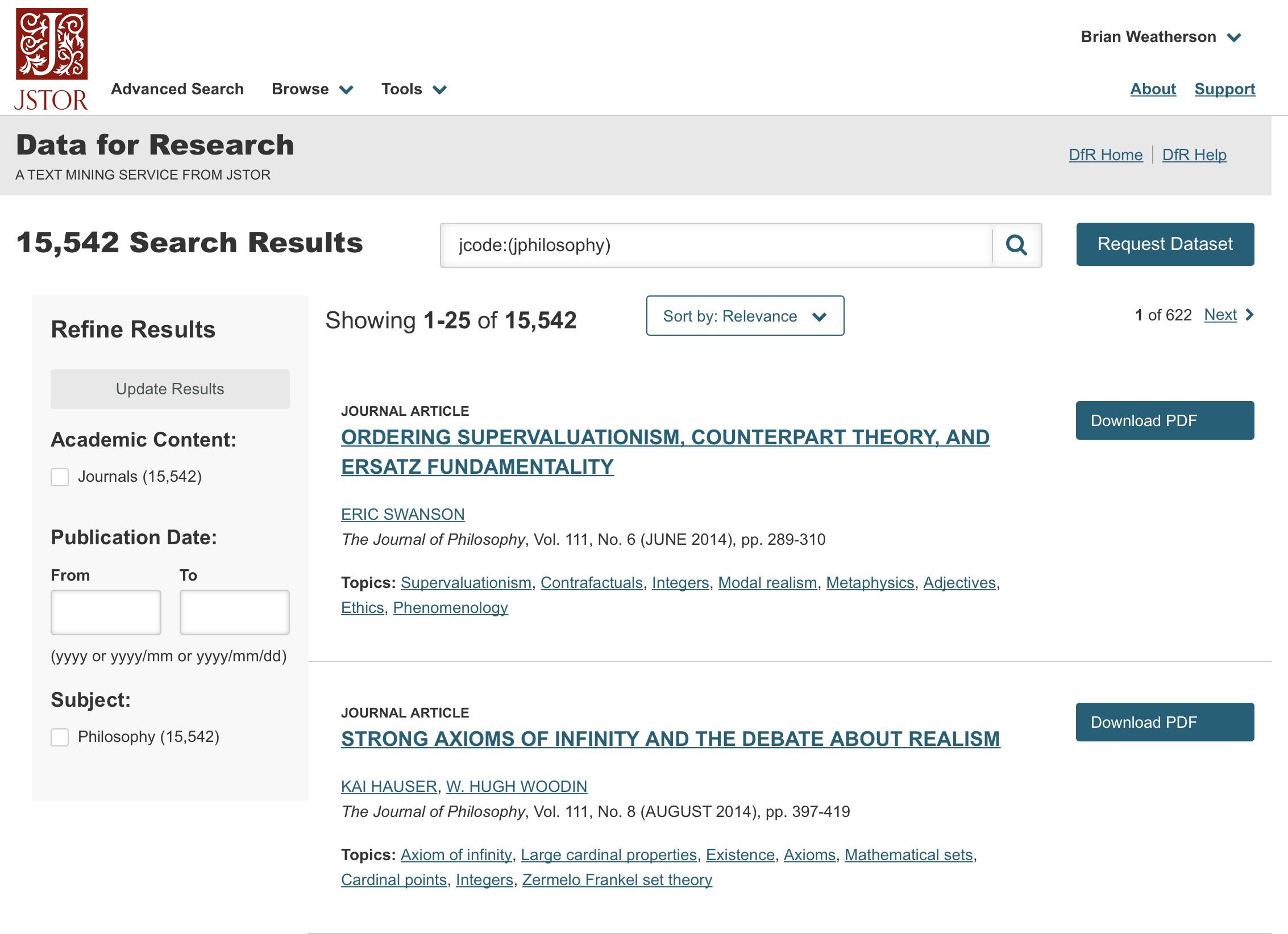
Finding all Journal of Philosophy articles

We are going to restrict dates, so let’s just do the 1970s. Type in the years you want, for us it’s 1970 to 1979, and click “Update Results”.

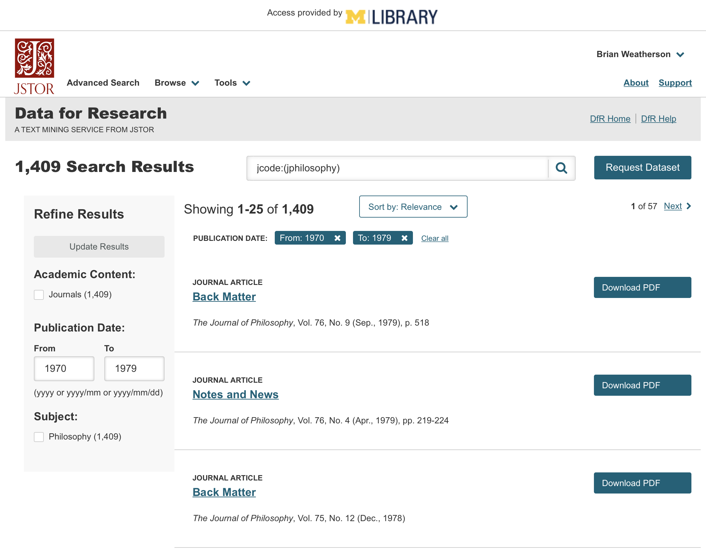
Restricting to the 1970s

Click “Request Dataset”. You need the metadata and the unigrams, and you need to give it a name (but you won’t use it at any time).

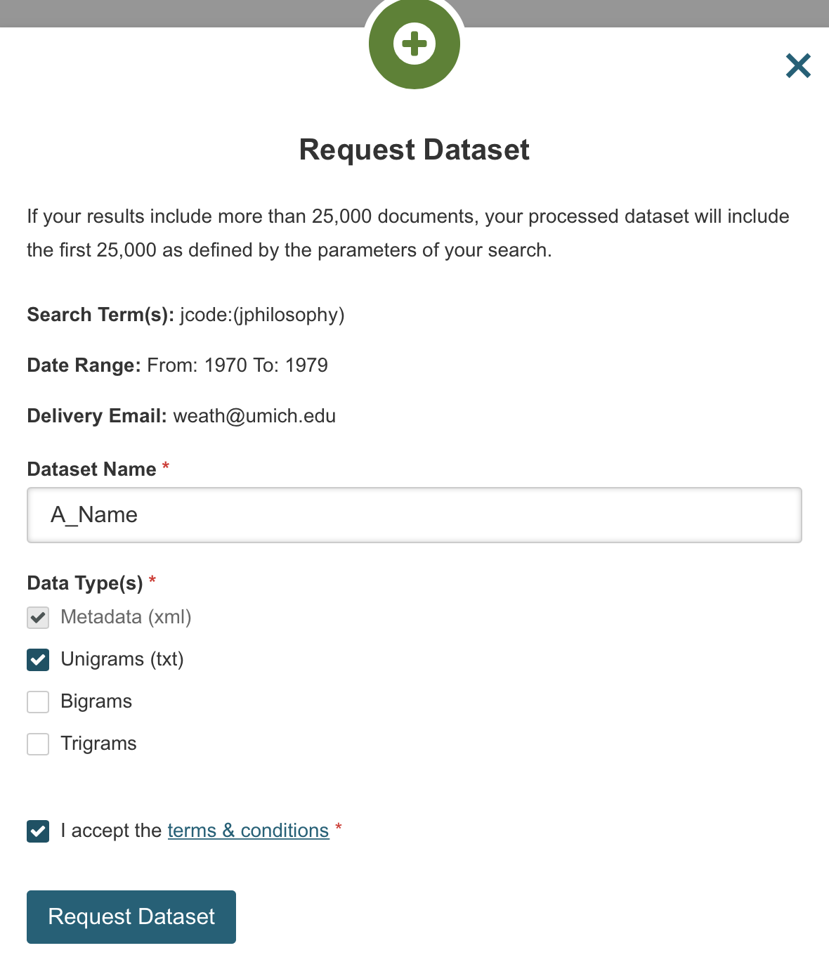
What data to get

Once again, click “Request Dataset”. You’ll get this somewhat less than reassuring popup.

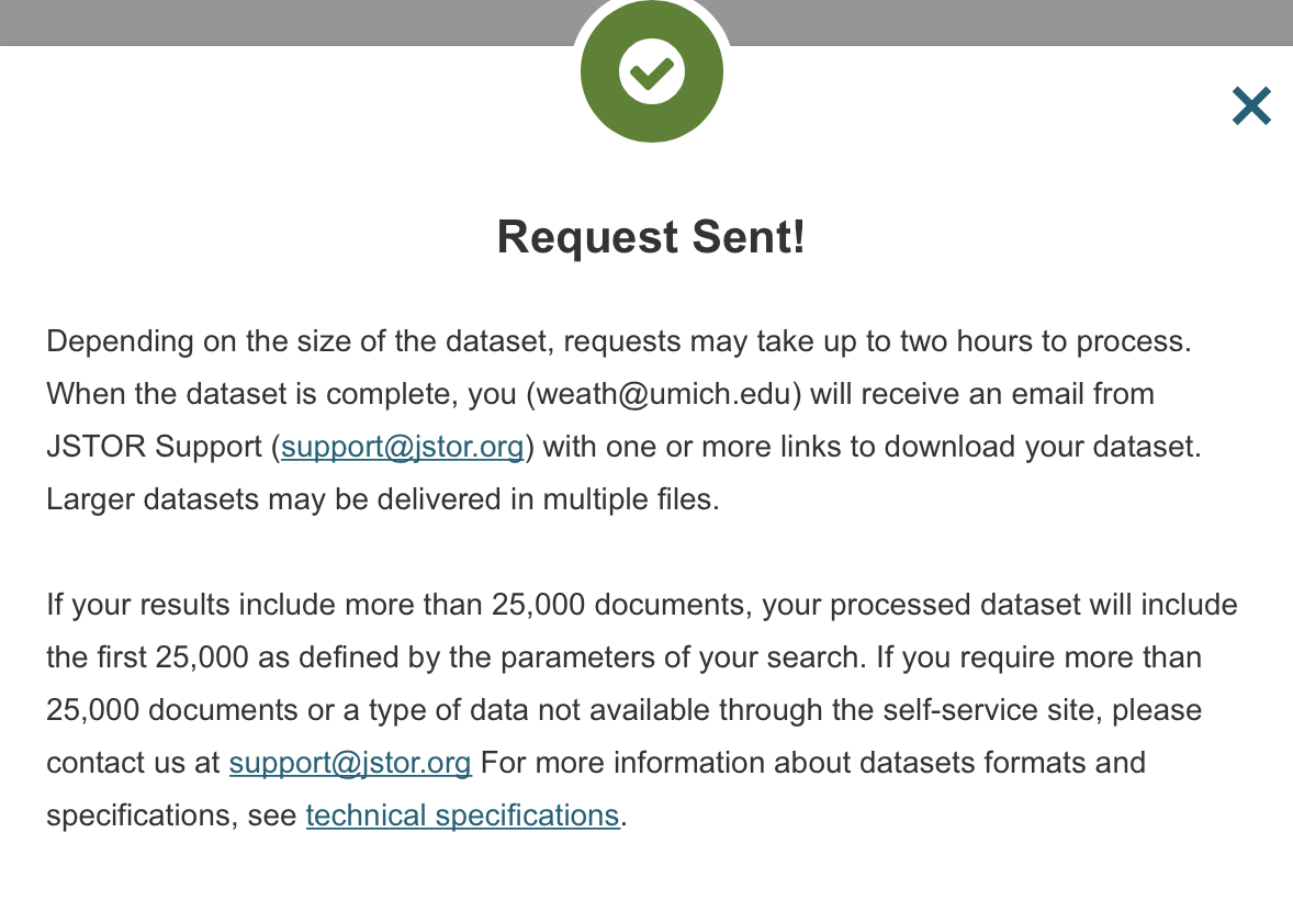
Uh oh—waiting time

But despite it saying that it may take up to two hours, in fact you normally get the data in minutes, even seconds. You’ll get an email (at the address you used for registration) saying it’s ready. Clicking the link in that email will get you a zip file. And in that zip file there are two directories: ngram1 and metadata.

We want to put these somewhere memorable. I’ll put the first in data/ngram/jphil and the second in data/metadata/jphil. (So data is a subdirectory of my main working directory. And it has two subdirectories in it, ngram and metadata. And each of those have a subdirectory for each journal being analyzed.) It’s good to keep the ngrams and the metadata in separate places, and it will be very useful (actually essential) to the code I’m about to run to use the same directory name for where a particular journal’s metadata is, and where its words are.

There is a hitch here that I should be able to figure out in R, but I couldn’t. As things come out, I ended up with names that didn’t have spaces in them. So the author of “Should We Respond to Evil with Indifference” was BrianWeatherson, not Brian Weatherson. There was probably a way to fix this at the importing stage, but doing so required more understanding of XML files than I have. So instead I came up with a hack. In each journal directory under inside metadata, go to the terminal and run this command:

find . -name '*.xml' -print0 | xargs -0 sed -i "" "s/<surname>/<surname> /g"

This adds a space before each surname. So in the surname field, that article goes from having the value “Weatherson” to having the value “ Weatherson”. And now it can be concatenated with “Brian” to produce a reasonable looking name. It’s not elegant, but it works.

The next two steps are taken almost entirely from John A. Bernau’s paper “Text Analysis with JSTOR Archives” (Bernau 2018). I’ve tinkered with the scripts a little, but if you go back to the supporting documents for his paper, you can see how much I’ve literally copied over.

Anyway, here’s the script I ran to convert the metadata files, which are in XML format, into something readable in R. The following file is called extract_metadata.R on the GitHub page. If you’re working with more journals, you have to add the extra journals into the tibble near the start. The first column should be the name you gave to the directories for the journal’s data; the second should be the name you want to appear in any part of the project being read by humans.

# Parsing out xml files
# Based on a script by John A. Bernau 2018

# Install / load packages
require(xml2)
require(tidyverse)
require(plyr)
require(dplyr)

# Add every journal that you're using here as an extra line
journals <- tribble(
  ~code, ~fullname,
  "jphil", "Journal of Philosophy",
)

all_metadata <- tibble()

journal_count <- nrow(journals)

for (j in 1:journal_count){
  
  # Identify path to metadata folder and list files
  path1 <- paste0("data/metadata/",journals$code[j])
  files <- list.files(path1)
  
  # Initialize empty set
  final_data <- NULL
  
  # Using the xml2 package: for each file, extract metadata and append row to final_data
  for (x in files){
    path <- read_xml(paste0(path1, "/", x))
    
    # File name - without .xml to make it easier for lookup purposes
    document <- str_remove(str_remove(x, ".xml"),"journal-article-")
    
    # Article type
    type <- xml_find_all(path, "/article/@article-type") %>% 
      xml_text()
    
    # Title
    title <- xml_find_all(path, xpath = "/article/front/article-meta/title-group/article-title") %>% 
      xml_text()
    
    # Author names
    authors <- xml_find_all(path, xpath = "/article/front/article-meta/contrib-group/contrib") %>%
      xml_text()
    auth1 <- authors[1]
    auth2 <- authors[2]
    auth3 <- authors[3]
    auth4 <- authors[4]
    
    # Year
    year <- xml_find_all(path, xpath = "/article/front/article-meta/pub-date/year") %>% 
      xml_text()
    
    # Volume
    vol <- xml_find_all(path, xpath = "/article/front/article-meta/volume") %>% 
      xml_text()
    
    # Issue
    iss <- xml_find_all(path, xpath = "/article/front/article-meta/issue") %>% 
      xml_text()
    
    # First page
    fpage <- xml_find_all(path, xpath = "/article/front/article-meta/fpage") %>% 
      xml_text()
    
    # Last page
    lpage <- xml_find_all(path, xpath = "/article/front/article-meta/lpage") %>% 
      xml_text()
    # Language
    lang <-  xml_find_all(path, xpath = "/article/front/article-meta/custom-meta-group/custom-meta/meta-value") %>%  
      xml_text()
    
    # Bind all together
    article_meta <- cbind(document, type, title, 
                          auth1, auth2, auth3, auth4, year, vol, iss, fpage, lpage, lang)
    
    final_data <- rbind.fill(final_data, data.frame(article_meta, stringsAsFactors = FALSE))
    
    # Print progress 
    if (nrow(final_data) %% 250 == 0){
      print(paste0("Extracting document # ", nrow(final_data)," - ", journals$code[j]))
      print(Sys.time())
    }
  }
  
  # Shorter name
  fd <- c()
  fd <- final_data
  
  # Adjust data types
  fd$type <- as.factor(fd$type)
  fd$year <- as.numeric(fd$year)
  fd$vol <- as.numeric(fd$vol)
  fd$iss <- str_replace(fd$iss, "S", "10") # A hack for special issues
  fd$iss <- as.numeric(fd$iss)
  
  # We are going to replace S with some large number, and then undo it a few lines later
  fd$fpage <- str_replace(fd$fpage, "S", "1000") 
  fd$lpage <- str_replace(fd$lpage, "S", "1000")
  # Convert to numeric (roman numerals converted to NA by default, but the S files should be preserved)
  fd$fpage <- as.numeric(fd$fpage)
  fd$lpage <- as.numeric(fd$lpage)
  fd <- fd %>%
    mutate(
      fpage = case_when(
        fpage > 1000000 ~ fpage - 990000,
        fpage > 100000 ~ fpage - 90000,
        TRUE ~ fpage
      )
    )
  fd <- fd %>%
    mutate(
      lpage = case_when(
        lpage > 1000000 ~ lpage - 990000,
        lpage > 100000 ~ lpage - 90000,
        TRUE ~ lpage
      )
    )
  fd$fpage[fd$fpage == ""] <- NA
  fd$lpage[fd$lpage == ""] <- NA
  
  # Create length variable
  fd$length <- fd$lpage - fd$fpage + 1
  
  # Convert to tibble  
  fd <- as_tibble(fd)
  
  # Filter out things that aren't research-article, have no author
  fd <- fd %>%
    arrange(desc(-length)) %>%
    filter(type == "research-article") %>%
    filter(is.na(auth1) == FALSE)
  
  # Filter articles that we don't want  
  fd <- fd %>%
    filter(!grepl("Correction",title)) %>%
    filter(!grepl("Foreword",title)) %>%
    filter(!(title == "Descriptive Notices")) %>%
    filter(!(title == "Editorial")) %>%
    filter(!(title == "Letter to Editor")) %>%
    filter(!(title == "Letter")) %>%
    filter(!(title == "Introduction")) %>%
    filter(!grepl("Introductory Note",title)) %>%
    filter(!grepl("Foreword",title)) %>%
    filter(!grepl("Errat",title)) %>%
    filter(!grepl("Erata",title)) %>%
    filter(!grepl("Abstract of C",title)) %>%
    filter(!grepl("Abstracts of C",title)) %>%
    filter(!grepl("To the Editor",title)) %>%
    filter(!grepl("Corrigenda",title)) %>%
    filter(!grepl("Obituary",title)) %>%
    filter(!grepl("Congress",title))
  
  # Filter foreign language articles. Can't filter on lang = "eng" because some articles have blank
  fd <- fd %>%
    filter(!lang == "fre") %>%
    filter(!lang == "ger")
  
  # Convert file to character to avoid cast_dtm bug
  fd$document <- as.character(fd$document)
  
  # Add a column for journal name
  fd <- fd %>%
    mutate(journal = journals$fullname[j])
  
  # Put the metadata for this journal with metadata for other journals
  all_metadata <- rbind(fd, all_metadata) %>%
    arrange(year, fpage)
}

save(all_metadata, file  = "my_journals_metadata.RData")

# The rest of this is a bunch of tweaks to make the metadata more readable

my_articles <- all_metadata

# Get Rid of All Caps
my_articles$title <- str_to_title(my_articles$title)
my_articles$auth1 <- str_to_title(my_articles$auth1)
my_articles$auth2 <- str_to_title(my_articles$auth2)
my_articles$auth3 <- str_to_title(my_articles$auth3)

#Get rid of messy spaces in titles
my_articles$title <- str_squish(my_articles$title)
my_articles$auth1 <- str_squish(my_articles$auth1)
my_articles$auth2 <- str_squish(my_articles$auth2)
my_articles$auth3 <- str_squish(my_articles$auth3)

# Note that this sometimes leaves us with duplicated articles in my_articles
# The following is the fix duplication code
my_articles <- my_articles %>% 
  rowid_to_column("ID") %>%
  group_by(document) %>%
  top_n(1, ID) %>%
  ungroup()

# Making a list of authors; uses 'et al' for 4 or more authors
my_articles <- my_articles %>%
  mutate(authall = case_when(
    is.na(auth2) ~ auth1,
    is.na(auth3) ~ paste0(auth1," and ", auth2),
    is.na(auth4) ~ paste0(auth1,", ",auth2," and ",auth3),
    TRUE ~ paste0(auth1, " et al")
  ))

# Code for handling page numbers starting with S, and for just listing last two digits in last page when that's all that is needed
my_articles <- my_articles %>% 
  mutate(adjlpage = case_when(floor(fpage/100) == floor(lpage/100) & fpage < 10000 ~ lpage - 100*floor(lpage/100),
                              TRUE ~ lpage)) %>% 
  mutate(citation = case_when(
    journal == "Philosophy of Science" & fpage > 10000 ~ paste0(authall," (",year,") \"", title,"\" ",journal," ",vol,":S",fpage-10000,"-S",lpage-10000,"."),
    journal == "Proceedings of the Aristotelian Society" & year - vol > 1905 ~ paste0(authall," (",year,") \"", title,"\" ",journal," (Supplementary Volume) ",vol,":",fpage,"-",adjlpage,"."),
#    TRUE ~ paste0(authall," (",year,") \"", title,"\" ",journal," ",vol,":",fpage,"-",lpage,".")
    TRUE ~ paste0(authall,", ",year,", \"", toTitleCase(title),",\" _",journal,"_ ",vol,":",fpage,"–",adjlpage,".")
  )
  )

# Remove Errant Articles
# This is used to remove duplicates, articles that aren't in English but don't have a language field, etc.
# Again, this isn't very elegant, but you just have to look at the list of articles and see what shouldn't be there
errant_articles <- c(
  "10.2307_2250251",
  "10.2307_2102671",
  "10.2307_2102690",
  "10.2307_4543952",
  "10.2307_2103816",
  "10.2307_185746",
  "10.2307_3328062"
)

# Last list of things to exclude
my_articles <- my_articles %>%
  filter(!document %in% errant_articles) %>%
  filter(!lang == "spa")

save(my_articles, file="my_articles.RData")

The main thing I added to this was the ugly code for handling articles with S in their page number. This doesn’t matter for the Journal of Philosophy in the 1970s. But two other journals have page numbers that look like S17, S145, etc. Treating these as numbers was a bit of a challenge, and the ugly code above is an attempt to handle it. As you can see, I’ve written distinct lines in for the two journals that I was looking at that did this; if you look at more journals you’ll have to be careful with this.

The other thing I did is right near the end, which is the mutate command that introduces the citation field. That’s a really helpful way of referring to articles in a familiar, human, and readable way. If you prefer a different citation format, that’s the line you want to adjust.

We now have a tibble, called my_articles that has the metadata for all the articles. It’s somewhat helpful in its own right; I use the large one I generated from all twelve journals for looking up citations. But we also need the words. For this I use another script that I built off one from Bernau’s paper.

This is called extract_words.R on the GitHub page. And again, if you want to use more journals, you’ll have to extend that tibble at the start.

# Read ngrams
# Based on script by John A. Bernau 2018
require(tidyverse)
require(quanteda)

# Journal List
journals <- tribble(
  ~code, ~fullname,
  "jphil", "Journal of Philosophy",
)

jlist <- journals$code

# Initialise huge tibble
huge_tibble <- tibble(filename = character(), word = character(), wordcount = numeric())

for (journal in jlist){
  # Set up files paths
  path <- paste0("data/ngram/",journal)
  n_files <- list.files(path)
  
  # Connecting Words to Filter out
  source("short_words.R")
  
  big_tibble <- tibble(filename = character(), word = character(), wordcount = numeric())
  
  for (i in seq_along(n_files)){
    # Remove junk to get codename
    codename <- str_remove(str_remove(n_files[i], "-ngram1.txt"),"journal-article-")
    
    # Get metadata for it
    meta <- my_articles %>% filter(document == codename)
    
    # If it is in article list, extract text
    if(nrow(meta) > 0){
        small_tibble <- read.table(paste0(path, "/", n_files[i]))
        small_tibble <- small_tibble %>%
          dplyr::rename(word = V1, wordcount = V2) %>%
          add_column(document = codename, .before=1) %>%
          mutate(digit = str_detect(word, "[:digit:]"),
                 len = str_length(word)) %>% 
          filter(digit == F & len > 2) %>% 
          filter(!(word %in% short_words)) %>% 
          select(-digit, -len)
        big_tibble <- rbind(big_tibble, small_tibble)
    }
    if (i %% 250 == 0){
      print(paste0("Extracting document # ", journal, " - ", i))
      print(Sys.time())
    }
  }
  huge_tibble <- rbind(huge_tibble, big_tibble)
}

# Adjust data types
my_wordlist <- as_tibble(huge_tibble)
my_wordlist$document <- as.character(my_wordlist$document)
my_wordlist$word <- as.character(my_wordlist$word)

save(my_wordlist, file  = "my_wordlist.RData")

Now with a tibble of all the articles, and another with all the words in each article, it’s time to go to work. The next file is called create_lda.R on the GitHub page, and if you’re doing a big project, it could take some time to run. This particular script takes less than a minute to run on my computer. But the equivalent step in the main project took over eight hours on a pretty powerful laptop.

require(tidytext)
require(topicmodels)
require(tidyverse)

# This is redundant if you've just run the other scripts, but here for resilience
load("my_wordlist.RData")
load("my_articles.RData")

source("short_words.R")

# Filter out short words and words appearing 1-3 times
in_use_word_list <- my_wordlist %>%
  filter(wordcount > 3) %>%
  filter(!word %in% short_words) %>%
  filter(document %in% my_articles$document)

# Create a Document Term Matrix 
my_dtm <- cast_dtm(in_use_word_list, document, word, wordcount)

# Build the lda
# k is the number of topics
# seed is to allow replication; vary this to see how different model runs behave
# Note that this can get slow - the real one I run takes 8 hours, though if you're following this script, it should take seconds
my_lda <- LDA(my_dtm, k = 10, control = list(seed = 22031848, verbose = 1))

# The start on analysis - extract topic probabilities
my_gamma <- tidy(my_lda, matrix = "gamma")

# Now extract probability of each word in each topic
my_beta <- tidy(my_lda, matrix = "beta")

The big step is the one that calls the LDA command. That builds the topic model. From here, your job is to just do analysis. But just to demonstrate what this finds, here is a quick look at what we found.

Table 0.2: Top articles in topic 3 in example LDA.

Article
Michael A. Slote, 1977, “Morality and Ignorance,” Journal of Philosophy 74:745–67.
Conrad D. Johnson, 1975, “Moral and Legal Obligation,” Journal of Philosophy 72:315–33.
Jules L. Coleman, 1974, “On the Moral Argument for the Fault System,” Journal of Philosophy 71:473–90.
Harry S. Silverstein, 1974, “Universality and Treating Persons as Persons,” Journal of Philosophy 71:57–71.
Lawrence Kohlberg, 1973, “The Claim to Moral Adequacy of a Highest Stage of Moral Judgment,” Journal of Philosophy 70:630–46.
Kenneth E. Goodpaster, 1978, “On Being Morally Considerable,” Journal of Philosophy 75:308–25.
David Gauthier, 1979, “Thomas Hobbes: Moral Theorist,” Journal of Philosophy 76:547–59.
William Neblett, 1974, “The Ethics of Guilt,” Journal of Philosophy 71:652–63.
Gregory W. Trianosky, 1978, “Rule-Utilitarianism and the Slippery Slope,” Journal of Philosophy 75:414–24.
P. H. Nowell-Smith, 1970, “On Sanctioning Excuses,” Journal of Philosophy 67:609–19.

These are the ten articles that our little example LDA gives the highest probability to being in topic 3. What’s topic 3? I guess ethics, from the look of those articles. We could check this by seeing which words have the highest probability of turning up in the topic.

Table 0.3: Topic 3 words.

Word
moral
one
good
may
philosophy
right
principle
must
even
morality

And that seems to back up my initial hunch that this is about ethics, or at least about morality. I’m going to stop the illustration here, because to go any further would mean doing serious analysis on a model that probably doesn’t deserve serious attention. But hopefully I’ve said enough here that anyone who wants to can get started on their own analysis.