8.10 Raw Counts and Weighted Counts
This section has two aims.
The first aim is to see if we can find a measure of how specialised a topic is. Intuitively, some topics are extremely specialized - only people working in quantum physics talk about quantum physics. But other topics cut across philosophy - everyone talks about arguments. Is there some way internal to the model to capture that notion?
The second is to cast some light on the relationship between the two ways of measuring topic size I’ve been using: raw count and weighted count. The raw count is the number of articles such that the probability of being in that topic is higher than the probability of being in any other topic. The weighted count is the sum, across all articles, of the probability of being in that topic. Mathematically, it is the expected number of articles in the topic.
I’ll start by looking at the relationship between the raw count and the weighted count for a single topic: modality. And then I’ll turn to see what happens when the focus expands to the other 89 topics. Start with two variables:
- \(r\), the raw count of articles in the topic. For modality, this is 370. That is, there are 370 articles that the model thinks are more probably in Modality than in any other topic.
- \(w\), the weighted count of articles in the topic. For modality, this is 370.51. That is, across all the articles, the sum of the probabilities that they are in modality is 370.51.
So these are fairly close, though as we’ll see, that’s not typical. (Indeed, I picked Modality to focus on because they were close, and I wanted to see how typical that was.) There is a third variable I’m going to spend a bit of time on. Focus on those 370 articles whose probablility of being in Modality is greatest. The model gives them very different probabilities of being in Modality. Here are two articles from the 370.
| Subject | Probability |
|---|---|
| Modality | 0.8215 |
| Causation | 0.0840 |
| Composition and constitution | 0.0554 |
| Minds and machines | 0.0205 |
| Subject | Probability |
|---|---|
| Modality | 0.1373 |
| Verification | 0.1196 |
| Value | 0.0977 |
| Idealism | 0.0542 |
| Analytic/synthetic | 0.0516 |
| Universals and particulars | 0.0494 |
| Chance | 0.0469 |
| Moral conscience | 0.0355 |
| Definitions | 0.0318 |
| Time | 0.0301 |
| Perception | 0.0290 |
| Physicalism | 0.0268 |
| Promises and imperatives | 0.0247 |
| Arguments | 0.0240 |
| Justification | 0.0208 |
| Dewey and pragmatism | 0.0206 |
| Life and value | 0.0204 |
These were not picked at random. The Bird article is the one the model is most confident is in modality, and the Keyt article is the one of the 370 that it is least confident about. (Honestly I think the model got this one wrong and is confused by Lewis.) There is a range of probabilities between those though.
Among the 370 articles that make up the raw count for modality, the average probability the model gives to them being in the topic is 0.3819917. (That’s a little under the midpoint between the Bird and the Keyt articles, but not absurdly so.) This is the value for modality of the third variable I’m interested in:
- \(p\), the average probability of being in the topic among articles that are more probably in that topic than any other.
Between \(r\), \(w\) and \(p\), there are three things that look like plausible specialization measures.
- Measure One
- Ratio of raw count to weighted count, \(\frac{r}{w}\).
- Measure Two
- Average probability of being in the topic among articles that have maximal probability of being in the topic, i.e.,\(p\).
- Measure Three
- What proportion of the weighted count comes from articles that are “in” the topic, i.e., \(\frac{rp}{w}\).
The first measure is intuitive because (as we’ll see) it places arguments right at the bottom of the scale. And that’s intuitively our least specialized topic.
The second measure is intuitive because it measures how confident the model is in its placement for articles that get maximal probability of being in a topic. And specialized topics should, in general, do well on this. We won’t find the model thinking that this article is most probably a quantum Physics article, but maybe jusy maybe it’s a social contract theory article, and maybe it’s a depiction article, so we should spread the probability around between those.
The third measure is intuitive for a similar reason. If a topic is specialized, it won’t pick up an extra 3 percent there or 5 percent there to its weighted count from articles in other topics. Most of \(w\) will come from articles “in” the topic, i.e., from the part of \(w\) that \(rp\) measures.
The second and third are obviously related, since \(p = \frac{rp}{r}\). In some sense, they are just different ways of normalizing \(rp\) to the size of the topic.
But intuitively all three should be related, since they all feel like measures of specialization. It turns out this isn’t quite right.
Let’s start with measure one, the ratio of raw to weighted count. This is something I talked a bit about back in chapter 2 when discussing two ways of measuring topic size.
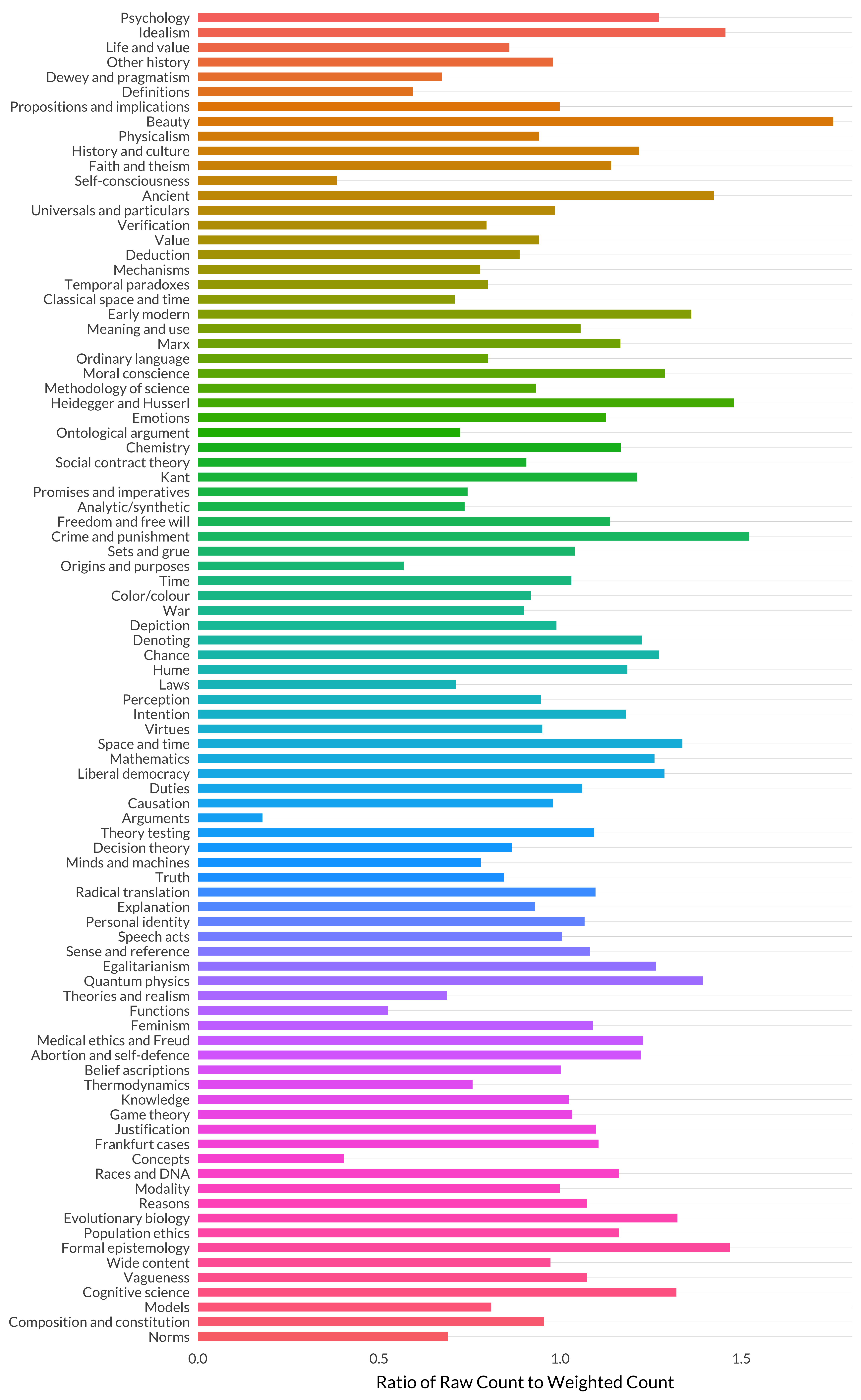
Figure 8.14: Ratio of raw count to weighted count by topic.
There is an enormous outlier here: arguments. (Though self-consciousness and concepts are also fairly low.) This makes sense—at least once the model decides that this will be a topic. There aren’t that many articles that are about arguments as such, but there are plenty of discussions of arguments in papers, so there are lots of ways to talk the model into thinking there’s a 2 or 3 percent chance that that’s the right topic for a particular paper.
To get a sense of how big the outliers are, it is useful to sort this graph by the ratio it represents.
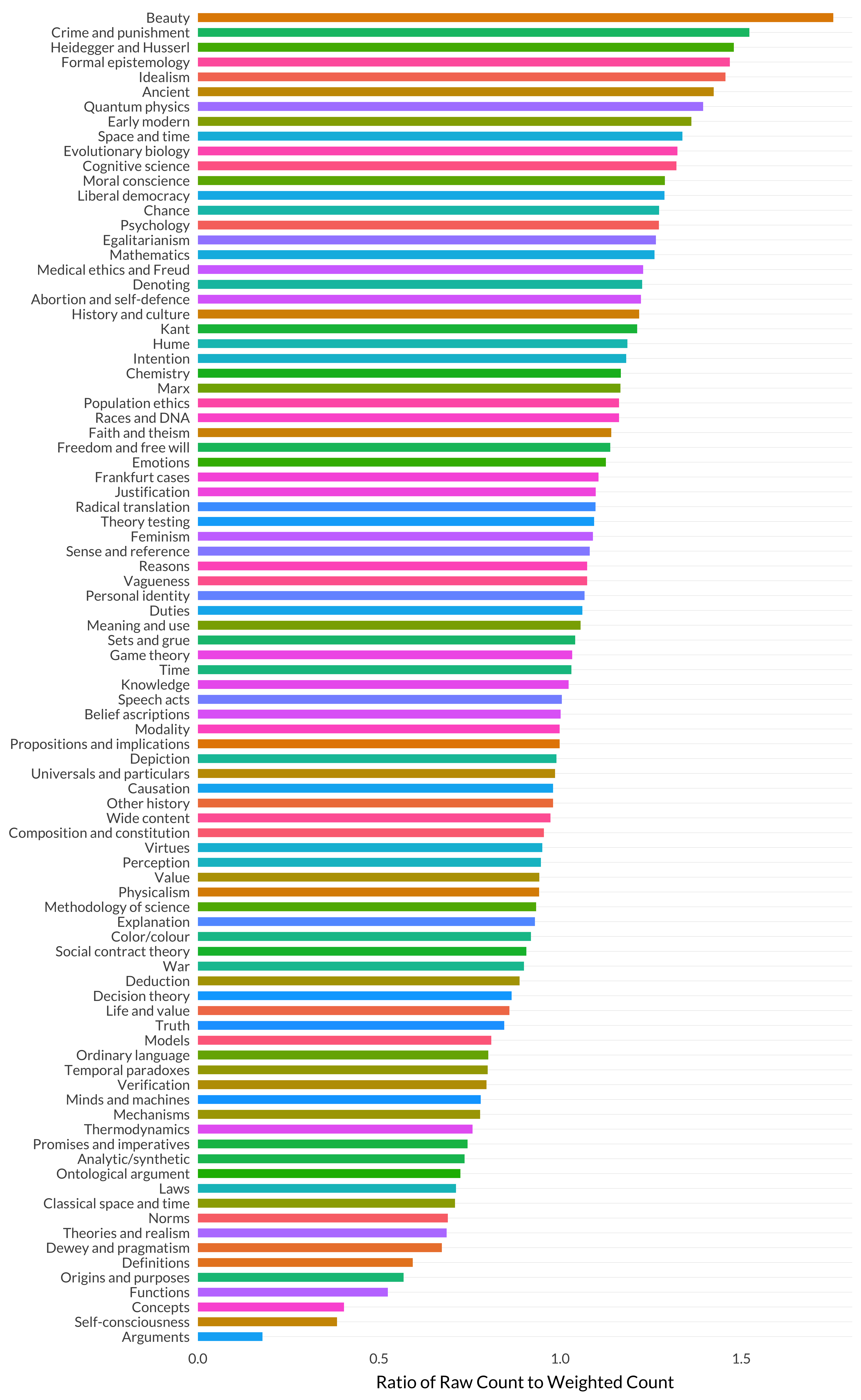
Figure 8.15: Ratio of raw count to weighted count by topic (sorted).
I don’t quite understand why beauty and crime and punishment are at the top of this graph. But I’ll keep a note of where beauty appears in subsequent graphs, because it is an interesting case.
Now we’ll look at the second measure, i.e., \(p\). For modality, the value of \(p\) is 0.3819917. How typical is that? Is the average maximal topic probability always around 0.4, or does it vary by topic? Let’s look at the data,, and note that the scale does not start at zero.
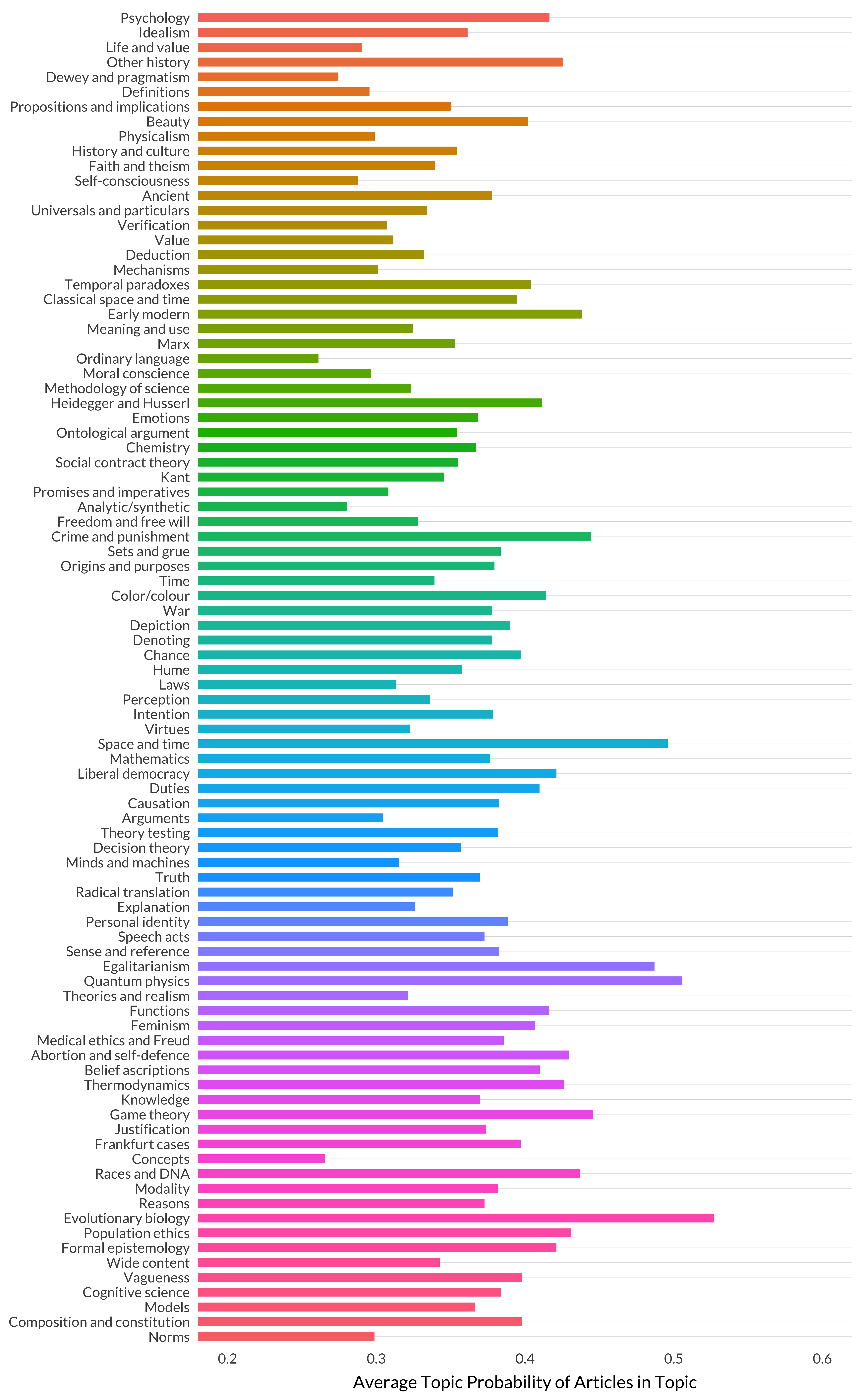
Figure 8.16: Average maximal probability by topic.
It turns out modality is reasonably typical, though there is a lot of variation here. Let’s look at the same graph but sorted by probability rather than topic number.
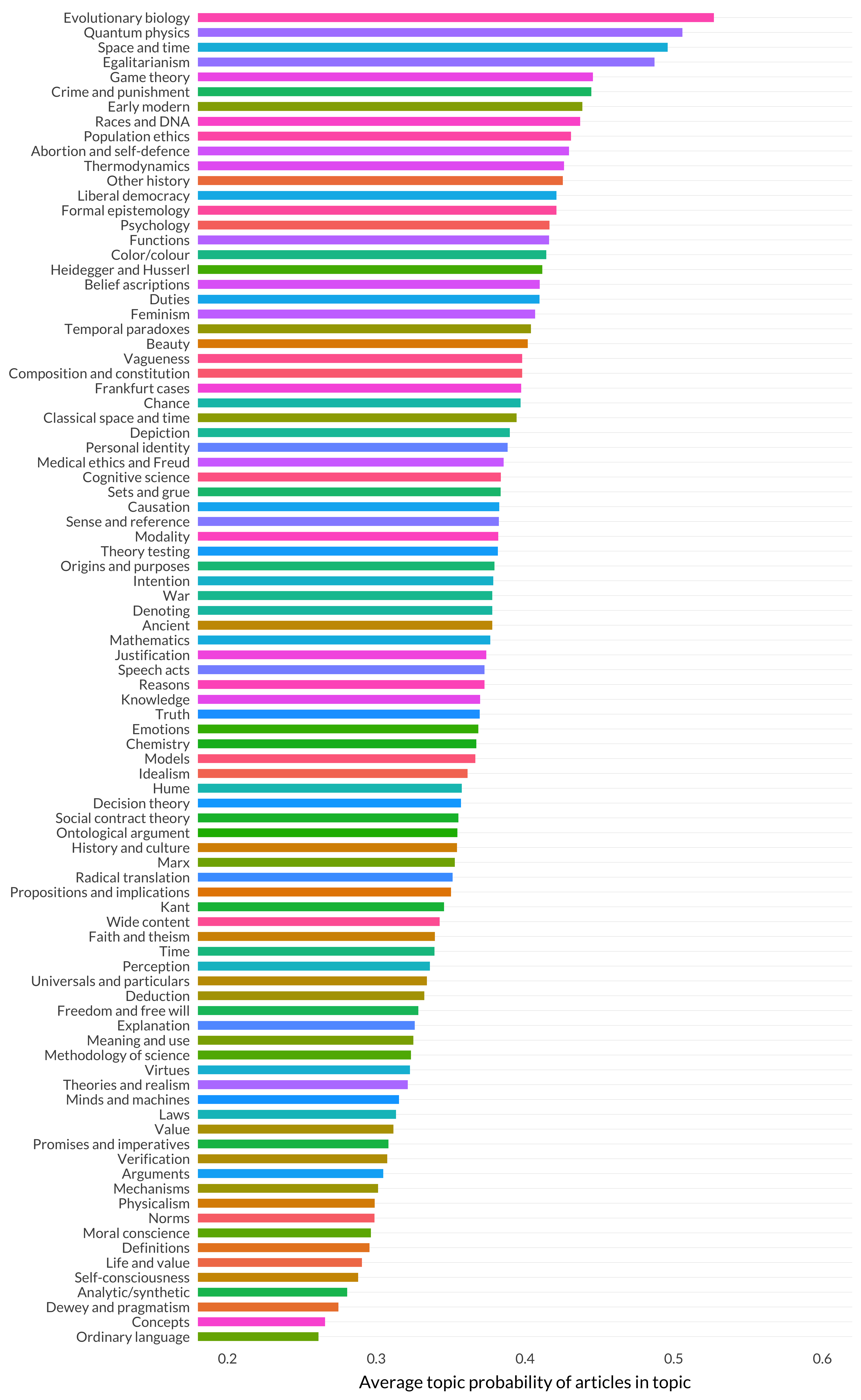
Figure 8.17: Average maximal probability by topic (sorted)
This does look like a measure of specialization. If a paper is talking about quantum physics or evolutionary biology, then it’s probably really talking about quantum physics or evolutionary biology. But lots of people use ordinary language and discuss concepts. So lots of articles that are about lots of different topics can end up looking like ordinary language or concepts articles.
Let’s turn to our last measure of specialization, \(\frac{rp}{w}\). One way to think about how big that is, is to think about the average probability of being in modality for the articles whose maximal probability is in one of the other eighty-nine topics. Some of these probabilities are quite large, such as for this article.
| Subject | Probability |
|---|---|
| Radical translation | 0.4538 |
| Modality | 0.4407 |
| Ontological argument | 0.0685 |
But most contributions aren’t that big. In fact, the average is under 1 percent. But there are nearly 32,000 of them, so they add up. In fact, they add up to about 61 percent of the weighted count for ,odality. So the value of \(\frac{rp}{w}\) for Modality is about 39 percent, since that’s what is left once you take out the 61 percent that comes from the rest of the articles. Is that 39 percent typical? Well, we can again look at the graph for all ninety topics.
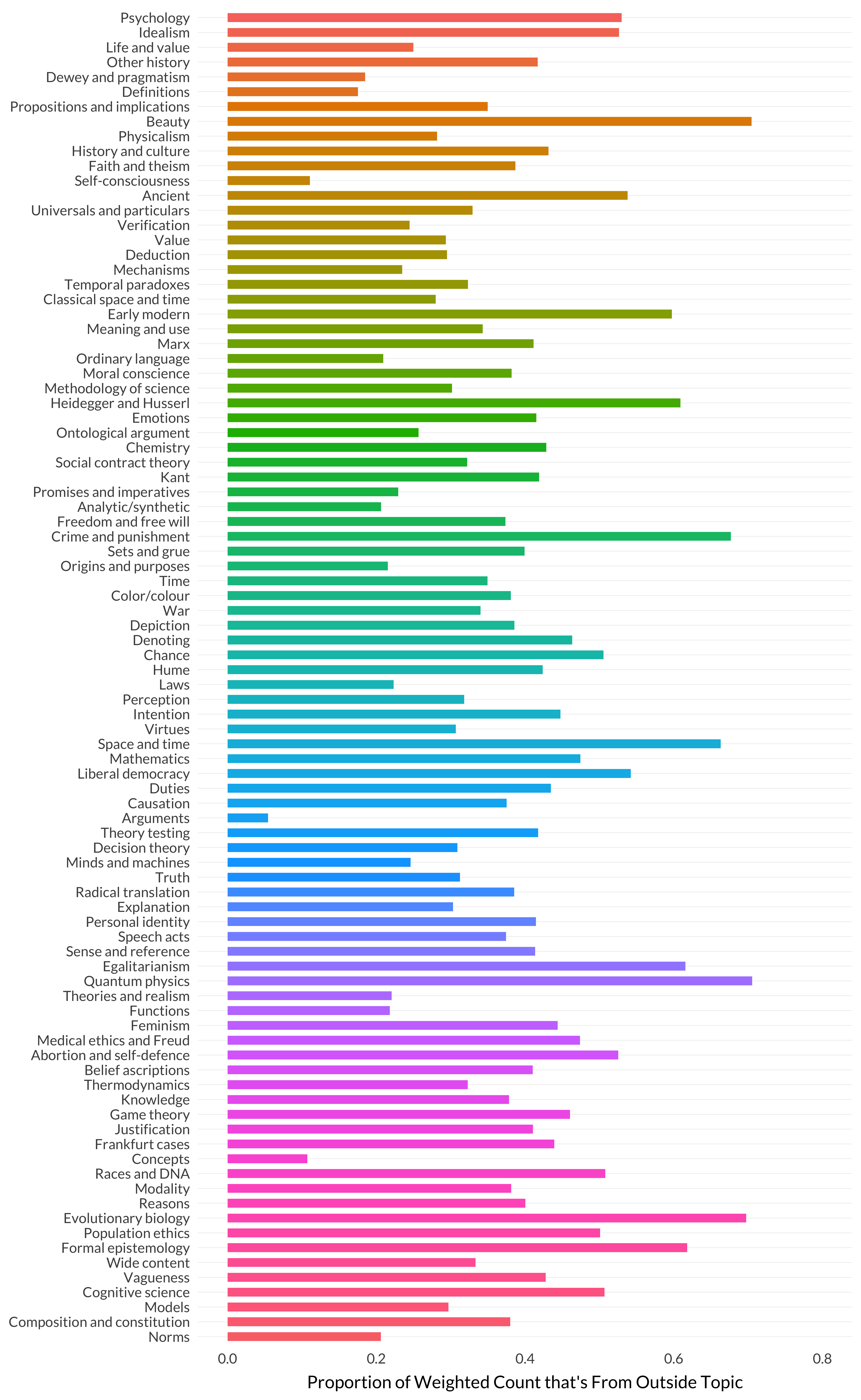
Figure 8.18: Proportion of weighted count that’s from non-topic articles.
And 39 percent is somewhat middling, though there’s so much variation that I’m not sure what I’d say is typical. Let’s look at that one arranged by order.
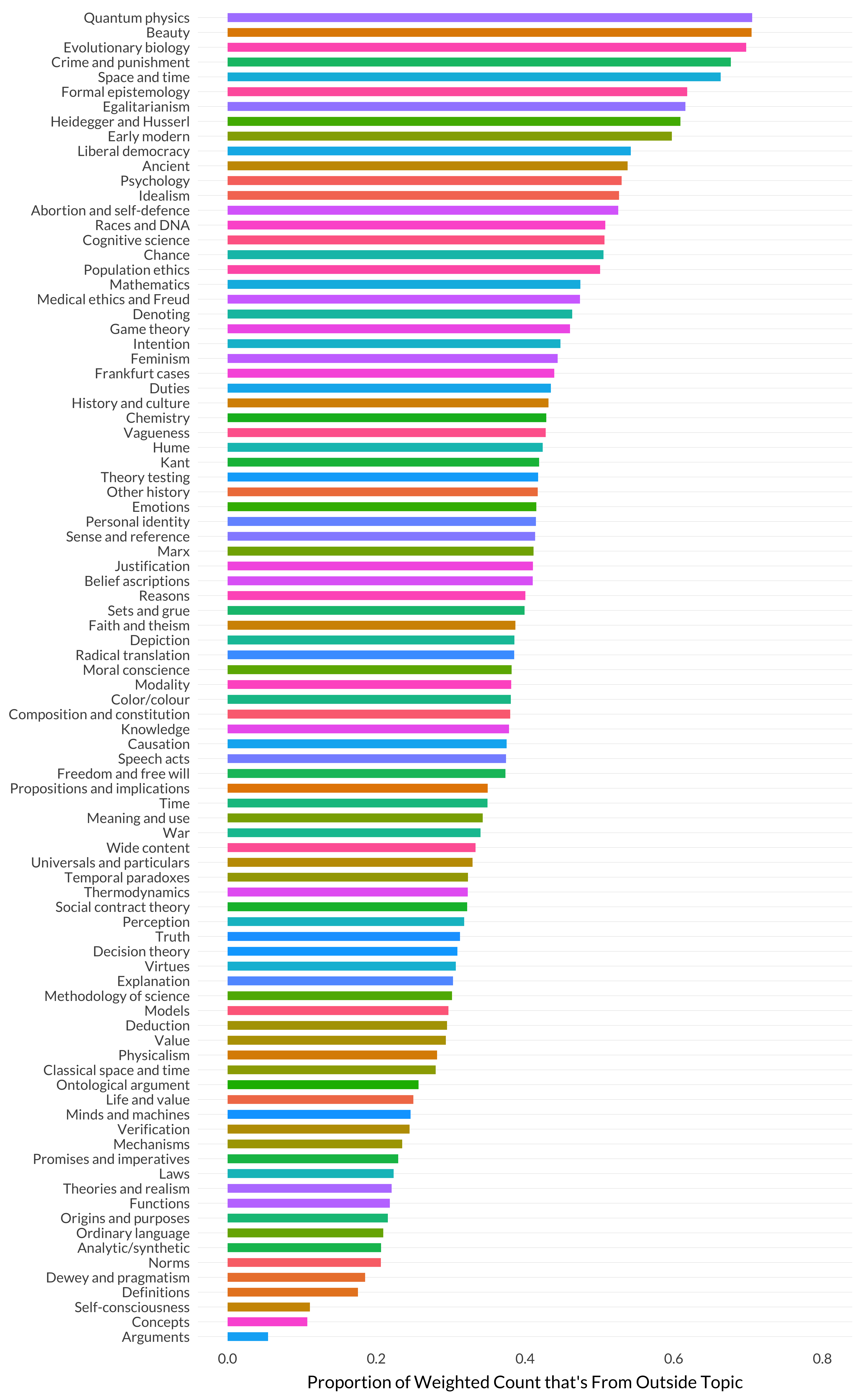
Figure 8.19: Proportion of weighted count that’s from non-topic articles (sorted).
And again, it looks like a measure of specialization. The model doesn’t give quantum physics much credit for articles that aren’t squarely about quantum physics. But it gives arguments lots of credit for articles that are not primarily about arguments.
If these three things are all sort of measures of specialization, they should correlate reasonably well. But this turns out not quite to be right. The first and second, for example, are not particularly well correlated. Here is the graph of the two of them, i.e., \(\frac{r}{w}\) and \(p\), against each other.
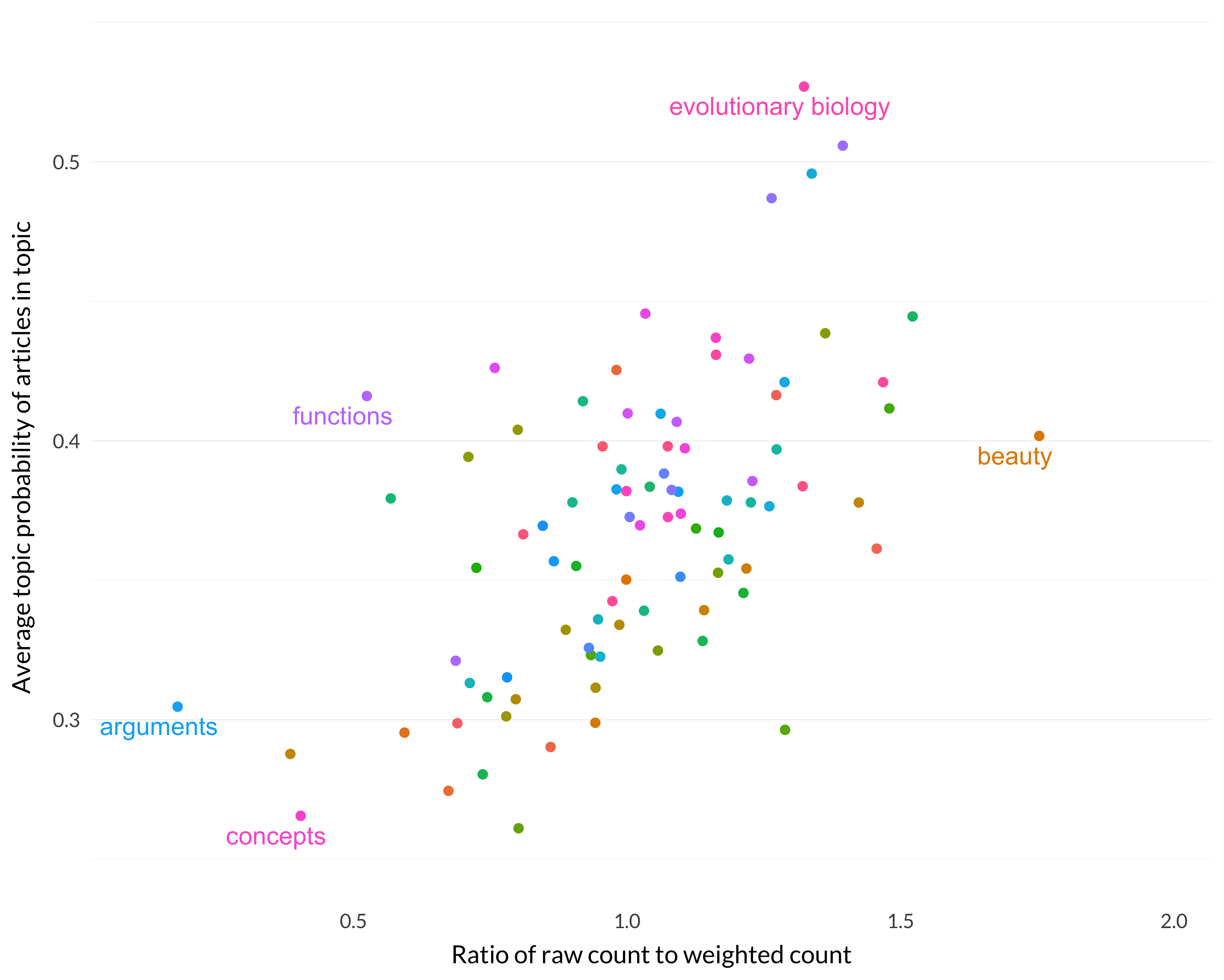
Figure 8.20: Correlation between the first and second specialization measures.
There is a trend there, but it’s not a strong one. But the other two pairs are much more closely correlated. (We have here a real-life example of how being closely correlated is not always transitive.) Here is the graph of the first against the third (i.e., \(\frac{r}{w}\) on one axis, and \(\frac{rp}{w}\) on the other).
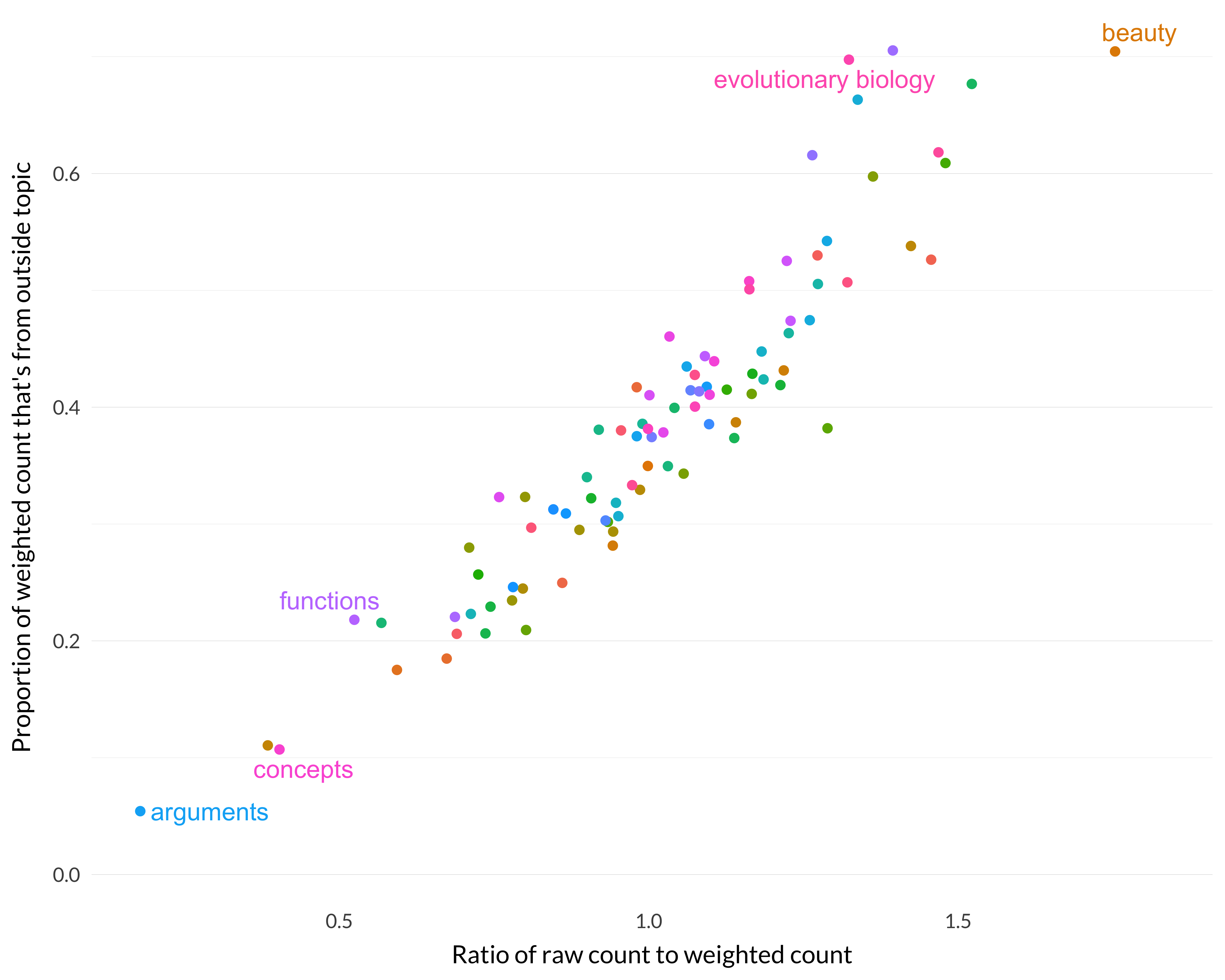
Figure 8.21: Correlation between the first and third specialization measures.
Interestingly, although those two are correlated, part of what that means is that there are some cases that they both misclassify if construed as measures of specialization. If we’re looking for a measure of specialization, we don’t want functions and evolutionary biology at opposite ends.
The last two measures, \(p\) and \(\frac{rp}{w}\) are also well correlated, though with some outliers.
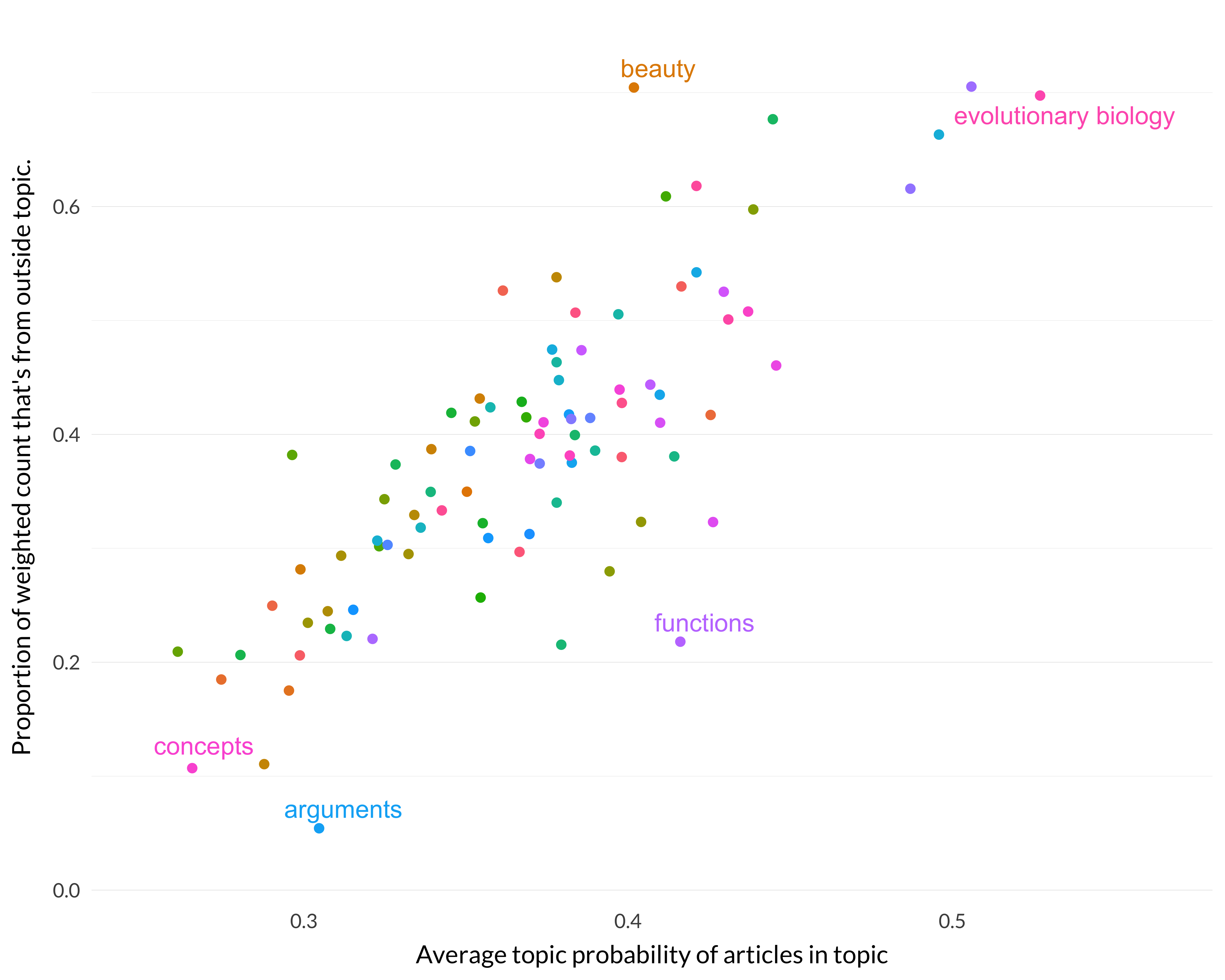
Figure 8.22: Correlation between the second and third specialization measures.
And our two measures of specialization do sort of line up. There are some outliers—functions is above the line and Beauty is below it.
I think that what we learn from that is that the best measure of specialization is \(p\), the average probability of being in the topic among articles whose maximal probability is being in just that topic. The other measures are roughly correlated with \(p\), but where they differ, \(p\) seems to do a better job of measuring specialization. And they are (somewhat surprisingly) very well correlated with each other.
And we also learned something about the relationship between \(r\) and \(w\). It’s really well correlated with \(\frac{rp}{w}\). And the best way to understand \(\frac{rp}{w}\) is to think about the average probability of being in a topic when that topic isn’t maximal. So \(r\) is low relative to \(w\) when a topic is often the second, third or fourth highest topic, and high when it is not. This isn’t surprising, but I had thought that this would in turn line up with how specialized a topic is. And that didn’t really do that. What did line up with intuitive specialization is the average probability of being in a topic among those papers where that topic probability is maximal.