PARTITION--Discrete

• Abstract--Contours
• Consider the scatter of dots with weights attached (often elevation).  Use a line to separate the scatter into three mutually exclusive and exhaustive sets:
• All values on the line are identical
• All values on one side of the line are less than the value along the line
• All values on the other side of the line are greater than the value along the line

Animated simple contouring of a scatter of irregularly spaced, weighted data.  There are an infinite number of ways that the contours can be placed between nearest neighbors--simple linear split or perhaps some sort of split representing concavity of the surface (in ArcView two common forms of interpolation involve "IDW" (Inverse Distance Weighted) or distance decay, and "spline" or "rubber sheeting" or minimizing total curvature).  Also, contours can be run off the edge of the page instead of wrapping across, as does the 1300 contour below.

• Use the geometric properties of partition to understand how to do contouring in ArcView (with Spatial Analyst Extension loaded).
• Link to base distribution of dots.  Load the .jpg as an image.  Use it as the base.
• From the base, create a new shape file of dots.
• Enter the first dot in the new shape file; open the attribute table of that shape file and add a column to it for elevation.  Add another dot to the shape file; enter the corresponding elevation in the table.  Continue editing the shape file and the table until all dots and elevations are entered.  Link to see the dot scatter in the shape file.  Link to see the attribute table of the dot scatter shape file.  Link to see the labelled shape file.
• Load the extension to ArcView called Spatial Analyst Extension.  Use the pull-down that has "create contours" on it (link).
• Contour the dot scatter using IDW and z-values from the appended column (elevation) in the attribute table (link).
• Contour the dot scatter using spline and z-values from the appended column (elevation) in the attribute table (link).
• The spline contouring appears more like the hand-contouring; where there is variation, it appears due largely to where one chooses to run a contour off the edge of the paper.  With the IDW contouring, it appears as if influence falls off quickly with distance and so there are a number of contours surrounding isolated nodes.

• Applied--Industrial Location (in the manner of Weber)
• Issue:  Cities are foci of agricultural consumption (marketplaces) and therefore have a strong influence on rural land use patterns.  Consider the parallel situation for industry.  Cities are marketplaces for industrial output.  What influence does that fact have on the location of facilities for resource processing and on consequent industrial location patterns?
• Simplifying Assumptions:
• Assume a uniform plane
• Assume a single urban market at a point
• Assume resources are point locations
• Assume equal transport costs per unit of weight
• Underlying Spatial Concept:  The point of lowest total transport cost will serve as an optimal location site for an industry.  This total is a sum of cost distances from resources and market.
• Mechanical model, Weber's weight analysis:  the accompanying figure shows a mechanical model of weights on strings.  Weights may represent cost in transport; the knot settles at the point minimizing total transport costs among the locations (holes) on the uniform (circular) plane region.
• Spatial Analysis:  Given one market, M, and two resource supply sites, R1 and R2
• Contour the plane surrounding each resource or market point according to transport costs from or to that point.  Given the simplifying assumptions, the pattern will be a set of concentric circles surrounding each point, evenly spaced, of increasing value as one moves outward from the resource site or marketplace.
• Model with equal transport costs (after Haggett)
• isotims:  contours of equal transport costs surrounding single points--see below for clear figure, using ArcView and buffers
• isodapanes:  contours of equal aggregate transport costs among a set of locations, inserted as dot scatter with weights calculated according to the isotim coordinate system.
• Model with unequal transport costs (modify the simplifying assumptions) (after Haggett)
• isotims:  contours of equal transport costs surrounding single points--see below for clear figure, using ArcView and buffers
• isodapanes:  contours of equal aggregate transport costs among a set of locations, inserted as dot scatter with weights calculated according to the isotim coordinate system.
• In both cases, an optimal location (according to the Underlying Concept) is found within the lowest contour on the resulting topographic map of isodapanes.
• Use ArcView to try to create the contours.
• Symmetric distance assumptions.
• Create a new shape file and draw three points in it (link).
• Enter a new column in the attribute table and enter the same elevation for each of the three points (900 in this case).
• Attempt to create contours using spline and the z-values in the new column; contouring will not occur because the surface is viewed to be flat since all values are equal in the z-value column of the attribute table (link).
• Try buffers.  Choose an interval of 100 feet.  Do not dissolve the buffers; then, one can see the circular coordinate system clearly.  The following map is created (link).
• Use the buffers in the previous set as a circular coordinate system. Insert a scatter of dots.  Measure the distance from each element of the dot scatter to the three purple dots.  Weight each element of the dot scatter with the sum of the distances.  Then, contour that dot scatter to create isodapanes.
• Assymetric distance assumptions.
• Create a new shape file and draw three points in it (link).
• Enter a new column in the attribute table and enter the same elevation for each of two of  points (900 in this case) and 1800 for the third point.
• Try buffers.  Choose an interval of 100 feet for the two points and 50 feet for the third.  Do not dissolve the buffers; then, one can see the circular coordinate system clearly.  The following map is created (link).
• Use the buffers in the previous set as a circular coordinate system. Insert a scatter of dots.  Measure the distance from each element of the dot scatter to the three dots.  Weight each element of the dot scatter with the sum of the distances.  Then, contour that dot scatter to create isodapanes.  The contours reflect the lack of symmetry and the stronger pull of higher transport costs to the one point.

• Abstract--Straight line

• Applied--Agricultural Land Use Model, von Thünen (based loosely (partially) on a description in Kolars and Nystuen)
• Simplifying assumptions:
• There is a single, isolated market at the center of the region
• The region is a homogeneous plain
• Labor costs are homogeneous
• Transportation costs are homogeneous
• The system is in economic equilibrium
• The market price of a single commodity is fixed.
• Fundamental Concept
Rent (as opposed to "rental"):  net return associated with a unit of land, rather than with a unit of commodity.
• Basic Spatial Conjecture
On any given parcel of land, the activity yielding the highest rent will dominate all others.
• Equations
• Net return, r, on a unit of commodity, given
p is the market price
c represents production costs
d is distance to market
t is transport rate
(hence, dt is total transport cost)
is:
r = p - c - dt
• Rent (net return), R, on a unit of land is given by r times the yield of the land (over a fixed time frame, such as a year).  If Y is the yield,
R = rY = Y(p - c) - Ydt.
Rewriting the equation, setting
P = Y(p - c), profit on amount of crop produced (market margin)
T = Yt, cost to ship the total amount of crop produced over one unit of distance
the equation becomes:
R = P - Td
• Implications of equations
• Whether the return is measured for unit of commodity or for unit of land, the measure of distance is invariant.
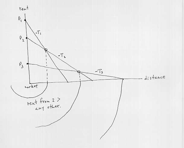
• In rewriting the rent equation, it becomes clear that the equation is of the linear slope-intercept form y = mx + b.  That is, rent is expressed as a linear function of distance R = f(d), in which the slope of the line representing the equation is -T and the intercept of the line with the vertical axis is P.  The units along the horizontal axis are "distance" and those along the vertical axis are "rent".
• Implications of the conjecture
• Different crops give rise to different equations, based on the idea that a given parcel will produce that which generates the greatest net return (and the variability of transport rates for different types of crops).
• Given an agricultural system with three crops:
R = P1 - T1 d
R = P2 - T2 d
R = P3 - T3 d
When the crop that yields the greatest rent is produced on all parcels of land, the resulting land use pattern is one of concentric circles centered on the market.
• Directions for extension
• Capture the ideas in software
• Test model against reality
• Vary the simplifying assumptions:  when, for example, is swamp reclamation feasible?
• Create non-linear split-domain Thünen functions
• Linear programming (simplex method) and the Thünen function. 

• References:
von Thünen, J. H.  von Thünen's Isolated State, trans. Carla M. Wartenberg, edited with an Introduction by Peter Hall, London: Pergamon Press, 1966.

Weber, Alfred.  Alfred Weber's Theory of the Location of Industries, trans. C. J. Friedrich.  Chicago:  The University of Chicago Press, 1928.

Puu, Tonu. Mathematical Location and Land Use Theory.  Springer-Verlag, 1997. 

Textbooks (out of print; contact instructor)
Kolars and Nystuen, Human Geography; 
Haggett, Peter, Geography:  A Modern Synthesis; 
Abler, Adams, and Gould, Spatial Organization.