Lecture Materials, UP507
(as a supplement to, not
a replacement for, in-class material.)
Week 1.
-
Introductions; project interests.
-
Website and syllabus
-
Biosketches: include background in GIS and project interests.
-
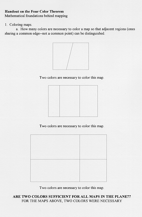
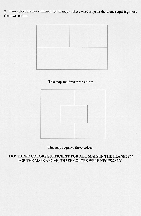
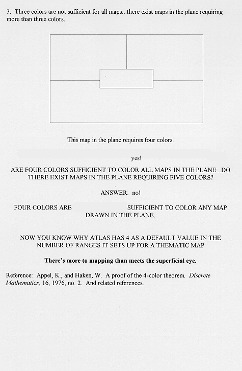
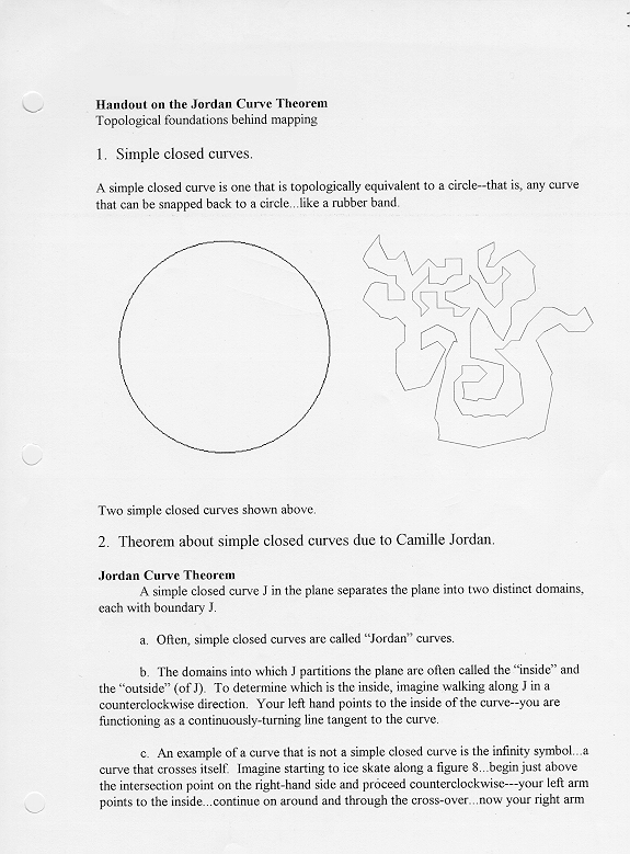
Given that no more than four colors are ever needed to color a map in the
plane, why should a GIS have so many choices for color?
-
Choropleth maps with many ranges need a variety of colors
-
Ranges need to make sense so that changes in data intensity are reflected
in changes in color intensity
-
Grayscale and color, this parallelism about data and color intensity is
critical
-
Four colors are sufficient to color any map in the plane; one never needs
more than four. Thus, when choosing coloring schemes, bear this fact
in mind and have a rationale for color selection based on the underlying
known theorem about coloring. One such good rationale is offered
above, involving choropleth maps.
-
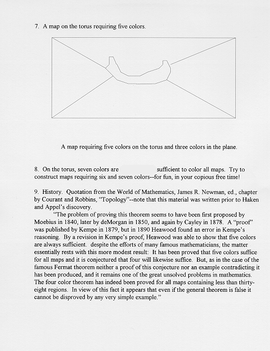
Open research questions: coloring issues with different forms of
polygon adjacency; coloring on different surfaces (some solved earlier--extra
reading: Page
4. Page
5. Page 6.Page
7. Six
color map). We may return to these later when we discuss map
transformations of various sorts.
-
Lab--set up website, discuss project interests.
Week 2.
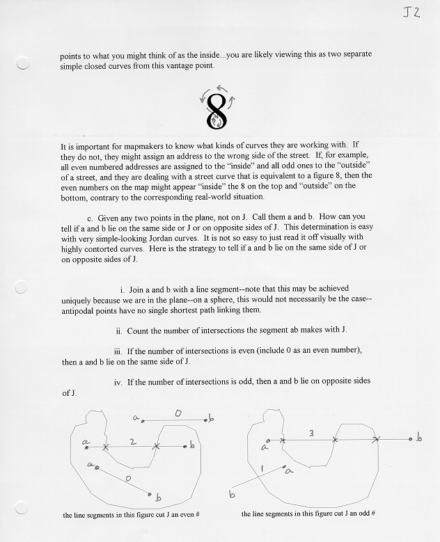
Jordan Curve Theorem; implications for mapping.
The Jordan Curve Theorem (click here
to see animated image of a walk in Lower Manhattan):
-
permits correct assignment of addresses on either
side of streets--suppose that the path is composed of two squares touching
at a point. When the path is separated into two squares, a consistent
assignment procedure for addressing may be given, such as the outsides
of the polygons have even numbered addresses on the north and the east
sides of streets and have even numbered addresses on the insides of polygons
on the south and the west edges of polygons. If the squares were
not split apart, then the south and west edges in this example would be
mislabelled. One must have the Jordan Curve Theorem built into the
software if geocoding is to work.
-
permits visually appropriate coloring of polygons
-
illustrates the need to split complex curves apart
at nodes where the curve crosses itself in order to ensure that the two
properties above will hold on maps. This fact is important in digitizing
(and elsewhere).
-
Lab: projects and websites.
Week 3.
-
Martin Luther King Day; office hours all afternoon;
no class.
Week 4.
-
Guest: Alan Levy, Director, Office of Neighborhood
Commercial Revitalization, City of Detroit.
-
Lab: projects and websites
Week 5.
Week 6.
Week 7. Focus on Spatial Transformations
-
Broad Concepts:
-
Map
scale
-
Latitude
and longitude (related reading: The Longitude; Mapping).
-
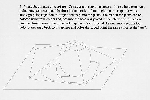
Map
projection: Stereographic projection.
The One-point Compactification Theorem (blackboard
demonstration):
shows that the skin of a spherical globe cannot
be perfectly flattened into the plane; it fails to do so by at least one
point. Thus, there can be no perfect map in the plane.
-
Four Colors are sufficient for any map on a sphere,
as well. An application of the one-point compactification theorem.
-
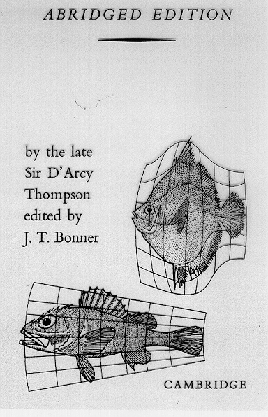
Map projection as a transformation: Thompson's
fish
-
Links
to various projections.
-
Geosystems
Handouts on Map Projections
-
Classification--move the center of projection; alter
the plane of capture (roll it up into a cylinder, torus, Möbius
strip, or Klein bottle--developable surface; try a cone).
-
Cylindrical and conical projections--choose a projection
suited to need.
-
Mercator--conformal--well-suited as a navigation
chart. Equal area projection better-suited to showing map of the
world.
-
Spider diagrams:
one way of defining regions in the absence of regional information.
-
Thiessen
polygons: another way of defining regions in the absence of regional
information
-
Contours:
Partitioning the plane in various ways.
-
Lab:
-
work on projects. Available on machines in my office: Animation
and other extensions.
-
Moving ArcView files...a time-saving maneuver
When moving a map from one computer to another, have you ever had the new
file ask you, over and over again, to locate all the shape files and .dbf
files? If so, consider the following approach, particularly when
there are many shape files in a single project. When you go to File|Save
Project As in ArcView, you create an .apr file that is a "project"
file. This file is a template that brings back the shape files you
chose with the themes colored the way you chose them to be colored, and
so forth. It is the
top level of a spatial hierarchy! The .apr file is a text file.
Text files can be edited in text editors, such as Windows NotePad. First,
open up the .apr file in ArcView and set the working directory to something
you want. Then, save the .apr file again, from ArcView. Next,
open up the .apr file in NotePad (it may ask to put the file in WordPad
if the file is too large--that is fine). Use the "find" command to
find the first occurence of "path c:\esri" or wherever the shape files
were saved. Then, use the replace command to replace c:\esri with
d:\esri (or whatever you need). You may or may not wish to use a
global replace command. You retain the most control simply by repeating
use of the "find" command and typing in suitable changes.
Week 8. Spring Break
Week 9. Midterm Presentations
Week 10. Guest: Karen Popek Hart, Planning Director, City
of Ann Arbor.
Week 11. Spatial Hierarchy and Fractal Transformations.
Week 12.
-
Finish material from week 11.
-
Break for 5 minutes
-
Number-theoretic properties were used to give precise information about
size and shape of fractal generator, above. In that case, knowing
the structure of the number completely determined the spatial result.
Numbers can also create spatial pattern. Consider the following locational
model of Hagerstrand.
-
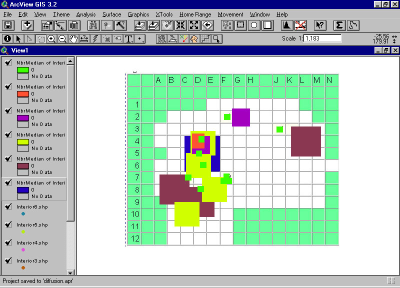
GIS software: The GIS may also be used to illustrate similar ideas:
spatial infill and extent.
-
Put down a dot for each adopter. Thus, one shape file has 22 dots.
-
Create a new field in the attribute table and insert associated random
numbers.
-
Partition these dots into the six different categories of the mean information
field.
-
Use "Analysis" | "Neighborhood Statistic" to build neighborhoods based
on position of cell in relation to center of MIF.
Week 13.
-
Perspective on conceptual material and its long-range importance
-
Short-range views--world wide web--huge resource
-
Standards for inclusion on the web
-
Copyright issues
-
eGovernment--using GIS and related software to build sites that permit
distribution of government records to a scattered population, requiring
no software other than what is routinely available in public libraries
and schools (a computer and an internet browser).
-
Favorite geographic resources--yours and mine.
-
Building a geographic archive--your wishes.
Week 14.
-
Building a geographic archive
-
One kind of strategy: SEMCOG model
-
Your wishes...
-
Guest speaker: John D. Nystuen--Water
Rustlers.
-
Classical cartography--hands on...
Week 15. Final Presentations.