Conceptual Material:  More of the MiniMax Principle
     Spatial analysis of many forms seeks to minimize one property (or set of properties) while maximizing another (hence, MiniMax).  One sees this principle in both conceptual and practical approaches. 
 

• Maximize contact between humans and natual landscapes in a minimum of terrestrial space with minimal environmental hazard.  Viewed in the context of condos along the Great Lakes's perimeter, one might ask how can individuals be offered the opportunity to secure desirable shore sites without doing extensive overall damage to vast stretches of shore line?  Fractal geometry offers one solution by compressing
• Mechanics of fractal construction

• Characteristics of the construction as applied to condos.
• Each condo pod has access to road on one side and shoreline on the other.
• Both road and water networks have successively narrower routes based on likely traffic--a hierarchy of widths
• The two network trees are separate from each other.  
• There are no bridges required
• Any one may have a tall-masted boat
• Infrastructure (pipes and so forth) is not exposed
• On

 

 
 

 
 
 
 
 

Graph Theory and Geography.

• Definition of a graph: 
A set of nodes V and edges E such that each edge is an undirected connection between two nodes. 
• The Königsberg Bridge Problem. 
• Link to map-statement of problem (from Arlinghaus, Arlinghaus, and Harary, Graph Theory and Geography:  An Interactive View, John Wiley and Sons, NY, in press, projected publication April , 2001); 
• link to graph.When the apparently complicated connection patterns were partitioned into the two categories, "regions" and "bridges," and then the regions represented as nodes and the bridges as edges, a graphical model of the problem emerged. Thus, it became possible for Leonhard Euler to show why such a walk was impossible. A trip of the sort desired by the townspeople is a sequence of nodes where each adjoining pair of nodes is joined by a different edge, and all seven edges are included. For example, A, D, B, C, A is a sequence starting and ending at A (returning to the

point of departure), but only four edges, AD, DB, one of BC, and one of CA, of the seven are included. In any such sequence of nodes and edges, at each node, an edge comes in and an edge goes out. Thus, the total number of edges at each node must be even (this number is called the degree of that node). In the multigraph of the Königsberg bridges, not just one but also all of the nodes have odd degree (Figure 1.4). Therefore, a traversal is impossible. 
• Euler's Theorem: 
A multigraph (graph with multiple edges joining at least one pair of nodes) has a traversal of the type mentioned (returning home and crossing each bridge exactly once) precisely when the degree of every node is even. 
• MiniMax: 
• Euler's Theorem might be used to construct or evaluate bus routes--"home" is the bus garage; the "nodes" are bus stops; the bridges are major arterials, bridges over freeways, etc.  If the route satisfies Euler's Theorem, then each major arterial or bridge is traversed exactly once in the course of the route, providing "maximal" service to riders with a "minimum" of gasoline use, congestion from buses, and wear on the buses.  Of course, that may not be an optimum set-up; sometimes redundancy is important.
• Euler's Theorem found actual application in constructing part of an algorithm for the Detroit Water Distribution Network--in helping to decide where to put redundant major connections.


Graph-theoretic Adjacency

• Graph-theoretic adjacency

1) Two nodes in a graph are adjacent if there is an edge joining them. 
2) Two nodes in a digraph are adjacent if there is an arc joining them.  If there is an arc from node u to node v, u is adjacent to v and v is adjacent from u. 
3) Two edges are adjacent if they are incident with a common node. 
• Adjacency matrix
• If a graph has n nodes, the adjacency matrix is an n x n matrix for which the entry in row i and column j is 1 if there is an edge (arc) from node i to node j and 0 if there is not. (The matrix is dependent on choosing an ordering of the vertices from 1 to n.) 
• Powering of matrices
• Application from British History:  drawing space and time together

More Specialized Adjacency

• Dot density maps:  layer of randomization, layer of observation--scale change; absolute representation (1 dot represents 1000 people) and relative representation (1 dot represents 0.1% of the population of the state).  Use ArcView.
• The concept of clustering is tied to scale.
• Equal Area Projections and dot density maps--one way to look for clustering in geographic space.
• First, select an equal area projection (such as an Albers Equal Area Conic for the U.S.).
• Next, select a distribution that can usefully be represented as dot scatter--such as population.
• Then, choose polygonal nets of at least two different scales--such as state and county boundaries.
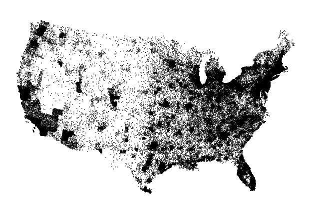
• Let the map with the smallest spatial units (counties) be used as the randomizing layer--the dot scatter is spread around randomly within each unit.
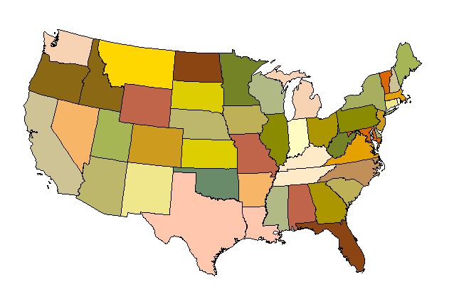
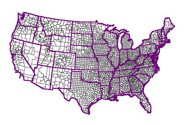
• View the scatter through polygons (states) that are larger than are those of the randomizing layer (counties).  Map 1 shows the results of removing the county boundaries; Map 2 shows the national picture with state boundaries; and, Map 3 views the dot scatter through the national border lens.  The clustering of dots at the state level means something; at the county level it is merely random.
• Because the underlying projection is an equal area projection, a unit square (or other polygon) may be placed anywhere on the map and comparisons made between one location and another.  Indeed, urban or rural measures might be held up to a value associated with similar polygon tossed out randomly.
Reference:  Mark Monmonier and Harm deBlij, How to Lie with Maps, University of Chicago Press.

• How are regions clustered in space?  Are similar ones next to each other or are dissimilar ones next to each other.  Consider for example some of the on-board population that comes with ArcView.  Open up the Michigan Block Group shape file.  Zoom in on southeastern Michigan.
• Go to Theme|Query;  click on the little "update values" box.  Then, double click on "black" then click on > then double click on "white". Choose "New Set".  Once the selected set comes up, go to to Theme|Convert to Shapefile.  Then, color the new shapefile with a green interior to produce this map of block groups in which quantity of black exceeds quantity of white.
• Go to Theme|Query;  click on the little "update values" box.  Then, double click on "white" then click on > then double click on "black".  Choose "New Set".  Once the selected set comes up, go to to Theme|Convert to Shapefile.  Then, color the new shapefile with a purple interior to produce this map of block groups in which quantity of white exceeds quantity of black.
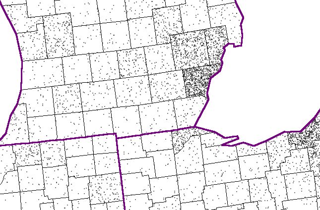
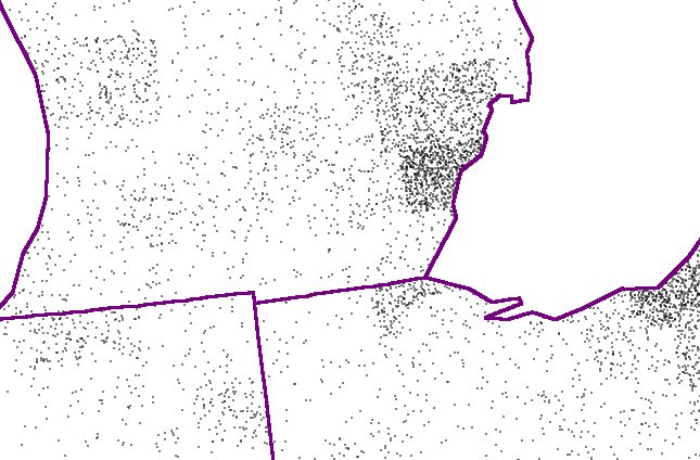
• A more detailed look at the clustering process might consider separating out those block groups in which black exceeds white and has a neighboring block group in which white exceeds black--denote this situation as BW.  There are then four logical alternatives:  BW, WB, BB, and WW.  On the maps, the Ws are always purple and the Bs are always green.  A deeper shade of purple represents a block group that is itself one in which white exceeds black and is one that has at least one neighboring block group in which black exceeds white.  To pick out the appropriate block groups:
• BW2:  make the B layer active. 
In ArcView 3.2: Go to Theme|Select by Theme.  In the top pull-down, select "are within distance of"; in the next pull down, select the W layer.  Then, for selection distance, choose 0 mi.  Choose "new set".  When the selected polygons come up, convert them to a shape file and color it a deeper green.  This process will pick out the edge of the B layer that is adjacent to the W layer.
• WB2:  make the W layer active. 
Go to Theme|Select by Theme.  In the top pull-down, select "are within distance of"; in the next pull down, select the B layer.  Then, for selection distance, choose 0 mi.  Choose "new set".  When the selected polygons come up, convert them to a shape file and color it a deeper purple.  This process will pick out the edge of the W layer that is adjacent to the B layer.
• Look at the whole map.  Clustering of like groups is evident in the Detroit metro area--similar groups are clustered.  In Washtenaw county some dissimilar groups are clustered, some are not.  Clustering of either similar or dissimilar groups is highest in Detroit--this would fit with field evidence.  This process can be iterated indefinitely (limited by the size of the base file) and creates yet another sort of "contouring".
• In terms of simple Medelian conditions, each of the four conditions,  BB, BW, WB, WW would be expected, with no constraints, to occur 25% of the time. 
• When all the block group outline boundaries are removed from the different colors, it is easy to look at a map of the whole state.
• Policy makers and municipal authorities may find maps such as these useful.
• Academic research may modify how to interpret what the adjacencies mean and what sort of quantitative significance to assign to them; it may also consider definitional matters, such as how polygons are adjacent--at corners only, at edges only, or at corners and edges.  Chess analogies are often-used jargon to describe such pattern.  The subject of "spatial statistics" delves more deeply into different measures for clustering and for levels of significance once clustering is found.