1. Questions often arise, after material is presented that involves intuitively sensible ideas of the projection of a wire globe to a physical surface, as to what else one might do. Here are a few projections that indicate what one might consider. Commentary based on material in Robinson and in Snyder.

a. The Sinusoidal projection (Sanson-Flamsteed projection)

In this projection, the non-central meridians are sine curves and the parallels and central meridian are straight lines. The spacing of the parallels and meridians are, to scale, the same as on the earth. The length of the central meridian is pi times the radius of the generating globe. The equator is twice the length of the central meridian. To construct the projection, draw an axis system with vertical axis pi times the radius of the generating globe, and horizontal axis twice that length; position the axes so that they are orthogonal and so that they bisect each other. Parallels are evenly-spaced and parallel to the equator (horizontal axis). The lengths of the parallels are the same as their lengths on the generating globe (to scale)---determined by multiplying the length of the equator by the cosine of the latitude. To see this, let R be the radius of the equatorial circle; the length of the equator is 2*pi*R. Let r be the radius of the small circle; its radius is 2*pi*r. Find r. Let a be the central angle in the sphere representing latitude. Draw the equator and small circle on a globe. Pass a meridian through them. Form angle a. From the ends of central angle a, draw the radii R and r in equator and small circle respectively. These two radii are parallel; the line forming the remaining side of angle a serves as a transversal to these two parallel lines. Because alternate interior angles are equal, angle a also is positioned between r and the other side. Draw the central axis of the sphere. Note the right triangles so formed. Thus cos a = r/R. Therefore,

R * cos a =r. Therefore, 2*pi*r = 2*pi*R*cos a = (2*pi*R)*cos a ; in the latter quantity, the value in parentheses is the length of the equator. Hence the original statement. Now, divide each parallel equally (with dividers...like a compass). Then, join the marks of division on each small circle with a French curve as a smooth curve. The nature of the construction makes it apparent that linear scale is correct along the parallels and the central meridian; it is the square root of the area scale and so there is no distortion of area scale.

This projection has been used in maps created at various times and locations. Cossin of Dieppe apparently used it for a world map in 1570; a bit later, it was used by Hondius for maps of Africa and South America that appeared in some of Mercator’s atlases and hence this projection is sometimes referred to as Mercator’s equal-area projection. Sanson d’Abbeville (1600-1667) used it for maps at the continental scale; Flamsteed (1646-1719), astronomer royal of England, used it for drawing charts of constellations.

b. Mollweide projection.

The sinusoidal projection is derived very simply from the sphere. The derivation of the Mollweide is not quite as straightforward. Because the meridians of the sinusoidal projection are sine curves, they intersect sharply at the poles and greatly compress the map as one moves close to the poles. Distortion is severe away from the equator, particularly as one moves away from the central meridian. The arithmetic properties of the Mollweide projection are similar to that of the Sinusoidal, but because the meridians are halves of ellipses (from one end of the major axis to the other), the compression at the poles is lessened. In this case, the length of the central axis is twice the square root of 2 (replacing pi) times the radius of the generating globe. The equator is, once again, twice the length of the central meridian. Beyond that, calculations involve constructing a circle inscribed in the eventual map boundary and determination of parallels and lengths of parallels based on relationships to this circle. Spacing between parallels is not even...it is successively narrower as one approaches the poles. Once the lengths and positions of the parallels have been determined, use of dividers and French curves proceeds as in the Sinusoidal.

Mollweide’s projection is an equal-area projection. Mollweide, a professor of mathematics and astronomy, announced it in 1805. Like the sinusoidal, it too has been used in a variety of applications--it appeared in numerous maps, both thematic and hemispheric, in Berghaus’s Physikalischer Atlas; it is also known as the Babinet, Homalographic, Homolographic, and elliptical projection. It has served as inspiration for a variety of 20th century global map projections, one of which is mentioned below.

c. Goode’s Homolosine (c. 1925)...and the beat goes on?

Goode combined the Mollweide (Homolographic) and the Sinusoidal to create the Homolosine...the poleward sections are Mollweide and the equatorial sections are sinusoidal. The two projections (when constructed to the same area scale) are joined along the one parallel they have of common length. The projection is generally displayed in interrupted form; central meridians were chosen to coincide with large land and ocean masses in order to reduce areal distotion. Some might find interrupted projections such as this a bit jarring; consider, however, that basically all maps are interrupted projections...they seem not to be jarring when the lines of interruption are at the edge of the map! Philbrick’s (1953) oblique view of the combined Sinusoidal and Mollweide produced a Sinu-Mollweide projection with smaller interruption north of the equator and depicting continuity of the landmasses in the northern hemisphere...
 
 

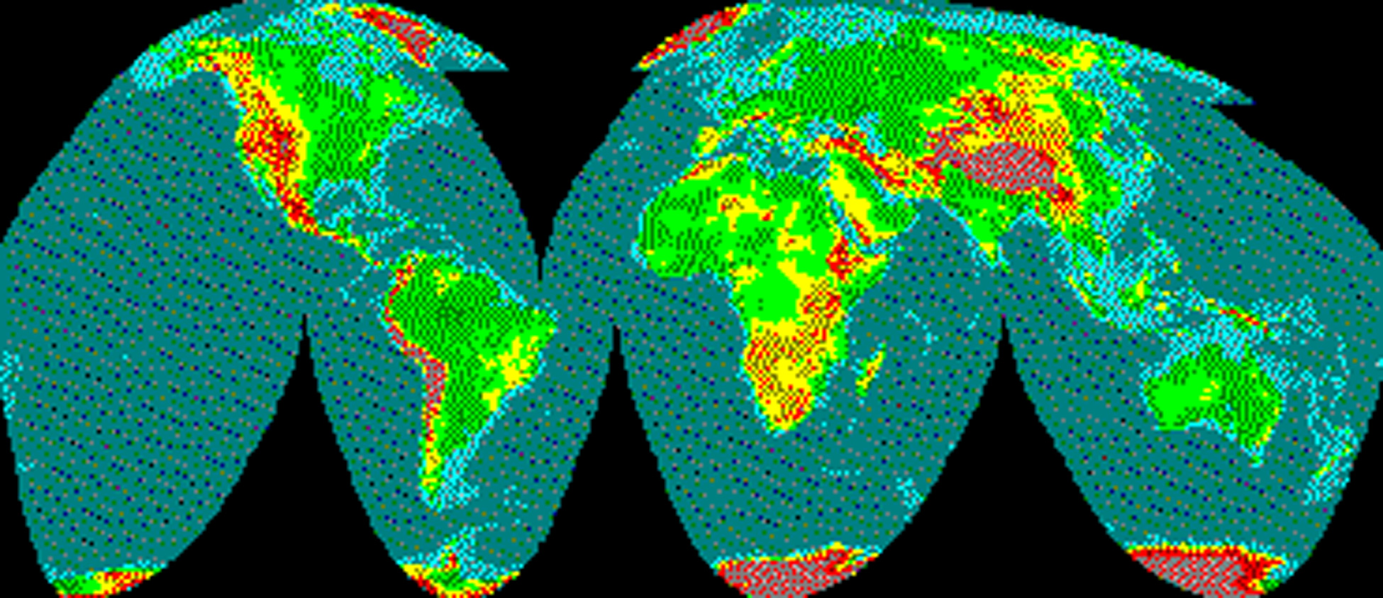
Goode's Homolosine: Sinusoidal from 40 N to 40 South; Homolographic (Mollweide) elsewhere.

From: This Human World, by Allen K. Philbrick, reprinted by Institute of Mathematical Geography.