We'll show that there's a relationship between some elementary geometry
of the plane and the Discrete Fourier Transform, then explore some ramifications of this for
polynomials, circulant matrices and interpolation ...
Elementary plane geometry was long a favorite of mathematicians and amateurs alike, but has fallen
a bit into disfavor nowadays. In the nineteenth century it was so popular a subject that
the comprehensive index of scientific papers put out by the Royal Society in London, England, explicitly
excluded over 600 papers on triangles and conic sections from its index volume for Pure Mathematics
which already comprised over 32,000 items.
It is of interest that one can view many of the theorems of plane geometry from a point of view
provided by the Discrete Fourier Transform (DFT) and that this leads on to some other results on
circulant matrices, smooth interpolation of point distributions in the plane, zeroes of polynomials,
and even a connection with quantum bits and the Heisenberg-Weyl algebra
as it turns up in signal processing.
In addition the geometric use of the DFT provides some beautiful diagrams for mechanical problems.
What is plane geometry? Start with the two-dimensional plane, which we'll think of as having
as coordinates complex numbers $x + \ii y \in \cplx$. Since theorems about
intervals defined by their two end-points are perhaps not too interesting, we'll start with the
geometry of triangles. There are several common classes of theorems about triangles.
I'll distinguish three types to begin with: Coincidence, Collinearity and Equilaterality.
Note the mathematical formula above. It is being displayed in your browser thanks to
the technology of Mathjax which has interpreted the
source of this article in which the formulas are input in $\TeX$. It could also have
handled MathML encoding.
Theorems of Coincidence
Triangle Medians
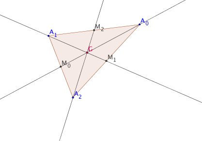
The first example is a triangle and the lines from the vertices to the bisection points
of opposite sides, which lines are called the medians. Pairwise, they intersect in 3 new points.
The first example theorem says these three points coincide. The point of common
intersection is called the centroid of the triangle. The figure below shows this.
The figures will often be accompanied by three options, Show, Hide
and Pop Up. The figure below is shown and can be hidden; if a figure is by default
hidden, it can be shown by clicking appropriately. Clicking Pop Up opens the interactive form
of a diagram in a separate small window. This can be left open along
with the article or closed in the way usual for a browser window. Note that the diagrams were
created with Geogebra and are Java applets, so that you must have a suitable version of Java
running to view them. In this first case we shall actually show the interactive diagram
to give a taste of what can be done. But later the illustrations will be fixed images
to make this article load faster.
Pop Up Diagram
This triangle has vertices $A_1$, $A_2$ and $A_3$. The points $M_1$, $M_2$ and $M_3$ are,
respectively, the midpoints of the sides opposite $A_1$, $A_2$ and $A_3$.
So the three medians are $A_1M_1$, $A_2M_2$ and $A_3M_3$.
The blue points $A_1$, $A_2$ and $A_3$ can be dragged with the mouse about to change
the form of the triangle, but $A_1M_1$, $A_2M_2$ and $A_3M_3$ remain
the medians of the resulting triangle.
The red point $G$, the triangle's centroid, actually marks the three coincident pairwise
intersections of $A_1M_1$, $A_2M_2$ and $A_3M_3$.
The axes are completely arbitrary and are there just for
familiarity.
Triangle Angle Bisectors
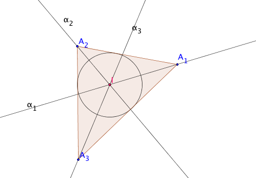
The second example is a triangle and the lines from the vertices that bisect the angles.
Pairwise, they intersect in 3 points. The second theorem says these three points coincide.
The point of coincidence is the the center of the incircle of the triangle.
Pop Up Diagram
The angle bisectors are the lines labelled $\alpha_1$, $\alpha_2$ and
$\alpha_3$, and the red point $I$ marks the three coincident pairwise
intersections of $\alpha_1$, $\alpha_2$ and $\alpha_3$ at the incenter.
The blue vertices $A_1$, $A_2$ and $A_3$ can be dragged about to change
the triangle in the interactive pop-up version.
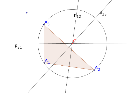
Triangle Perpendicular Bisectors
A third example is a triangle and the lines that perpendicularly bisect the sides.
Again the pairwise intersections coincide, at the circumcenter $C$.
Pop Up Diagram
The lines $p_{12}$, $p_{23}$ and $p_{31}$ are the respective perpendicular bisectors
of the triangle sides $A_1A_2$, $A_2A_3$ and $A_3A_1$.
Pairwise, they intersect in 3 points. The theorem says these three points
coincide as the red point $C$, the circumcenter.
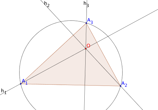
Triangle Altitudes
Again we have a coincidence for the altitudes of a triangle, the lines drawn from the
vertices perpendicular to the opposite sides. The point of coincidence is called the orthocenter.
Pop Up Diagram
The lines $h_{1}$, $h_{2}$ and $h_{3}$ are the
respective altitudes from $A_1$, $A_2$ abd $A_3$. Pairwise, they intersect in 3 points.
The theorem says these three points coincide as the red point $O$, the orthocenter.
Note that it is not the center of any particular circle we have already identified,
but it is the intersection of perpendiculars dropped from points on the circumcircle to
the opposite sides of the triangle, which are chords of that circle.
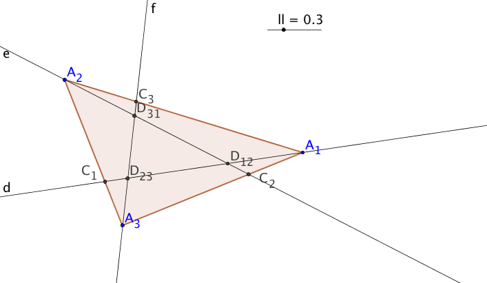
Triangle Cevians
Just to show that not every natural construction leads to a coincidence of pairwise intersetions,
note this is not so for arbitrary Cevians of a triangle, which are lines from the vertices
to points on the opposite sides.
Pop Up Diagram
The case illustrated in the diagram is that in which the
point on the opposite side is a constant proportion of the way along from each vertex to the
next one in the cycle $A_1$, $A_2$ , $A_3$. The initial case in the diagram is for the proportion
$\frac13$ but this can be adjusted with the slider at the top right of the diagram by dragging
the point along. Remark that for the value $\frac12$ we are back at the first case above
of Triangle Medians, and we do have coincidence.
Coincidence theorems
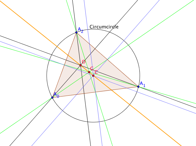
The prime example of a coincidence theorem is probably that concerning the Euler line.
The remarkable fact, first noted by Euler, is that the circumcenter $C$, the centroid $G$
and the orthocenter $O$ are collinear for any triangle with vertices $A_1$, $A_2$ and $A_3$.
The medians are in green and the perpendicular bisectors in blue.
The line through them is shown in orange so as to stand out a bit in the figure below.
Pop Up Diagram
Equilaterality theorems
Napoleon's Theorem
Napoleon's theorem, though probably not directly due to the emperor
himself, has long been eponymous with him. In its simplest form it
says that if one constructs on each side of a nondegenerate plane
triangle, and external to it, an equilateral triangle of base equal
to the side, and then takes the three centroids of the resulting
triangles, then these points are the vertices of an equilateral
triangle. That is you start with an arbitrary triangle, construct
three new points in a specified way and the resulting points are the
vertices of an equilateral triangle. This is illustrated in the
accoompanying diagram, which actually shows that a similar construction
using triangles on the other sides of the triangle sides also leads
to a different equilateral triangle.
Pop Up Diagram
The case illustrated in the diagram is that in which the
point on the opposite side is a constant proportion of the way along from each vertex to the
next one in the cycle $A, B , C$. The initial case in the diagram is for the proportion
$\frac13$ but this can be adjusted with the slider at the top right of the diagram by dragging
the point along. Remark that for the value $\frac12$ we are back at the first case above
of Triangle Medians, and we do have coincidence.
There is a rather more general form of the theorem which
will be seen as a consequence of what will be proved below. It states that
the results of a whole class of constructions which are specified to
be made on the edges of an arbitrary nondegenerate plane $N$-gon
will be a regular $N$-gon of a specific type.
Morley's Theorem
What was hailed when it was discovered as the first really new advance in plane
geometry since the Greeks became known as Morley's Miracle. It was found in about
1900 but not really published by its discoverer Frank Morley until many years
later. Many proofs of it have appeared, a notable recent one of great generality
being due to Alain Connes. It can be thought to be related to the approach
explored below.
Morley's basic concistruction is: F
or any non-degenerate triangle consider the internal angle trisectors. Then consider
the pairwise intersections of adjacent ones. The resulting points are the vertices of
an equilateral triangle. Again a diagram shows the remarkable assertion nicely.
Pop Up Diagram
The case illustrated in the diagram is that in which the
point on the opposite side is a constant proportion of the way along from each vertex to the
next one in the cycle $A, B , C$. The initial case in the diagram is for the proportion
$\frac13$ but this can be adjusted with the slider at the top right of the diagram by dragging
the point along. Remark that for the value $\frac12$ we are back at the first case above
of Triangle Medians, and we do have coincidence.
There is even more to be found from considering angle trisectors of
which there are two for each angle; indeed at each vertex there are
two angles the internal and the external. By considering all suitable
combinations of angles and trisectors, in fact one finds $18$ equilateral
Morley triangles assocciated to a given triangle. Liouville and others
later went on to consider other fractions of polygon angles and more
general constructions. Again a diagram can help.
Pop Up Diagram
The case illustrated in the diagram is that in which the
point on the opposite side is a constant proportion of the way along from each vertex to the
next one in the cycle $A, B , C$. The initial case in the diagram is for the proportion
$\frac13$ but this can be adjusted with the slider at the top right of the diagram by dragging
the point along. Remark that for the value $\frac12$ we are back at the first case above
of Triangle Medians, and we do have coincidence.
A pentagon construction
A new twentieth-century type of construction, that was devised probably around 1940
but only published in 1960 in a piece in honor of a colleague Jekuthiel Ginsburg, is due to
the American Fields medalist Jesse Douglas.
Consider a pentagon in the plane. For that matter, we could let the points be in a space of dimension
up to 4, since 5 points can only subtend a space of at most dimension 4. However, the formalism
is simpler for the plane so that's where we'll start. The full situation will be considered later.
We are viewing the 2-dimensional plane as given
by a single complex coordinate $z = x + \ii y$. Suppose the five vertex points are $ p_1$, $p_2$,
$p_3$, $p_4$, and $p_5$; so we are given the complex vector in ${\mathbb C}^5$, a list of points,
$$ p=(p_1,p_2,p_3,p_4,p_5).$$
Since no one point of the five is distinguished, we shall consider the indices $i$
of $p_i$ modulo $5$: sums in the index are cyclic, so that, for instance, $p_{3+4} = p_2$.
Douglas suggests: Join each vertex $p_i$ to the midpoint of the edge opposite between the
points $p_{i+2}$ and $p_{i+3}$ ; then extend that line by an extra piece of length
$(1/\sqrt{5})$ of the original piece to create a new vertex $q_i$. Douglas observed that
the new pentagon $(q_1, q_2, q_3, q_4, q_5)$ is always the affine image of a convex regular
pentagon. He also remarked that if, instead, the lines to the opposite midpoints are shortened
by a similar decrement ratio of $(1/\sqrt{5})$ to give new vertices $r_i$, then
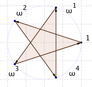
$(r_1, r_2, r_3, r_4, r_5)$ is the affine image of a regular star pentagon, commonly called a pentagram.
We interpret this in coordinates and plot sample results. We start with, say,
$ p=(p_1,p_2,p_3,p_4,p_5)$. The plots are done using an arbitrarily chosen example, but
as usual the vertices can be dragged about in the figure.
$$
p=(1.3 + 2.2 \ii, 4.4 + 1.5 \ii, 6 + 5.5 \ii, 1.5 + 4.1 \ii, 5.6 + 6.4 \ii).
$$
Pop Up Diagram
We see $$q_i = p_i + \left(1+\frac1{\sqrt{5}}\right)\left({\frac{1}{2}}(p_{i+2}+p_{i+3}) - p_i\right) ,$$
Pop Up Diagram
and similarly that
$$r_i = p_i + \left(1-\frac1{\sqrt{5}}\right)\left({\frac{1}{2}}(p_{i+2}+p_{i+3}) - p_i\right) .$$
Pop Up Diagram
Putting all this into a diagram with all the lines drawn, which it is amusing to pull about to see
the effectiveness of the construction, we get
Pop Up Diagram
Geometry with the Discrete Fourier Transform
The pentagon construction explained
Why does the above work? It can be explained by examining this construction with a really
simple example of what can be thought of as a Geometrical Fourier Transform. In this case
it's the Discrete Fourier Transform of order 5.
Let $\omega_k$ be the simplest primitive $k$th root of unity:
$$
\omega_k = \cos\frac {2\pi}k+ \sin\frac {2\pi}k \ii.
$$
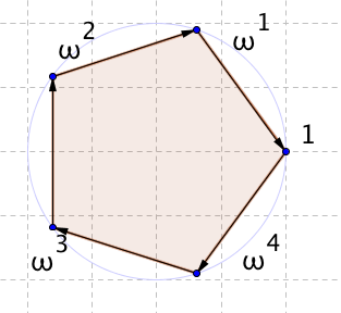
The standard convex regular pentagon can be taken to be the ordered set of points
$$
(\omega_5^0,\omega_5^1,\omega_5^2,\omega_5^3,\omega_5^4) =(1,\omega_5^{\strut},\omega_5^2,\omega_5^3,\omega_5^4).
$$
The standard regular star pentagon, or pentagram, can be taken to be the ordered set of points
$$
(\omega_5^{2\times0},\omega_5^{2\times1},\omega_5^{2\times2}, \omega_5^{2\times3},\omega_5^{2\times4})
=(1,\omega_5^2,\omega_5^4,\omega_5^1,\omega_5^3),
$$
which is the result of taking every other point starting from $1$. Note that complex conjugation
acts as $\overline{\omega_5^j} = \omega_5^{5-j}$.
We'll do the case $n=5$ of the starting construction first, so take $\omega := \omega_5^{\strut}$
until further notice. Remark also that
$$\cos\frac{2}{\pi}5 = \cos 72^\circ = \frac{1}{4} (-1+\sqrt5)\simeq 0.309, \quad \sin\frac{2}{\pi} 5
=\cos 18^\circ = \frac{1}{4}\sqrt{10+2\sqrt5} \simeq 0.951 .
$$
In fact, in terms of square roots,
$$
\left(
\begin{array}{c}
1\\
\omega_5^{\phantom{1}}\\
\omega_5^2\\
\omega_5^3\\
\omega_5^4
\end{array}\right) =
\frac{1}{4}
\left(
\begin{array}{c}
4\\
-1+\sqrt5 + \ii \sqrt{10+2\sqrt5}\\
-1-\sqrt5 + \ii \sqrt{10-2\sqrt5}\\
-1-\sqrt5 - \ii \sqrt{10-2\sqrt5}\\
-1+\sqrt5 - \ii \sqrt{10+2\sqrt5}
\end{array}
\right)
$$
$$=
\frac{1}{4} \left\{\, \left[
-\left(
\begin{array}{c}
1\\
1\\
1\\
1\\
1
\end{array}
\right)
+\sqrt5\,
\left(
\begin{array}{c}
\sqrt5\\
+1\\
-1\\
-1\\
+1
\end{array}
\right)
\,\right] +
\frac{\ii}{2} \sqrt{10+2\sqrt5}\,
\left[\,\,
\left(
\begin{array}{c}
0\\
2\\
1\\
-1\\
-2
\end{array}
\right)
+\sqrt5\,
\left(
\begin{array}{c}
0\\
0\\
-1\\
1\\
0
\end{array}
\right) \,
\right]\, \right\}
$$
which seems complicated enough.
Going back to examine the coordinates for $q_i$ we see
$$q_i = -\frac{\sqrt5}5 p_i + \frac{5+\sqrt5}{10} p_{i+2}+ \frac{5+\sqrt5}{10} p_{i+3}.$$
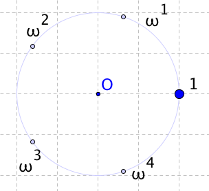
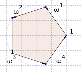
To establish properties of the shape of a pentagon we try to see what components of the
various standard types it has. The general fact is that any plane pentagon can be written
as a linear superposition, with complex coefficients, of the standard polygonal forms
with $5$ points. The 5 basic forms are:
a degenerate collection of five superposed points,
the standard regular convex pentagon,
the standard regular star pentagon,
the reversed regular star pentagon,
the reversed regular convex pentagon.
‘Standard’ means
consisting of points on the unit circle, and ‘reversed’ means the standard form described
in the opposite orientation. We will also refer to the reversed forms of the figures
as their opposites, since they have the opposite orientation. The four non-degenerate
types are illustrated below.
The coordinates of the five basic forms of a pentagon are: $$
(
1,
1,
1,
1,
1
)
\,,\quad(
1,
\omega_5^\strut,
\omega_5^2,
\omega_5^3,
\omega_5^4
)
\,,\quad(
1,
\omega_5^2,
\omega_5^4,
\omega_5^\strut,
\omega_5^3
)
\,,\quad(
1,
\omega_5^3,
\omega_5^\strut,
\omega_5^4,
\omega_5^2
)
\,,\quad(
1,
\omega_5^4,
\omega_5^3,
\omega_5^2,
\omega_5^\strut
)
$$
We shall consider a pentagon $p$ as a
function on the cyclic group ${\mathbb Z}/5 {\mathbb Z}$. In fact that's what we began to do as
soon as we adopted the convention that the indices were to be viewed modulo $5$.
The decomposition of a given pentagon into its standard components is just an example of
harmonic analysis for the cyclic group ${\mathbb Z}_{/5} := {\mathbb Z}/5 {\mathbb Z}$.
This is known as the Discrete Fourier Transform of order $5$.
The 5-dimensional space, ${\mathbb C}{\mathbb Z}_{/5} $,
known as ${\mathbb C}{\mathbb Z}_{/5}$'s complex group algebra,
of ${\mathbb C}$-valued functions on
${\mathbb Z}_{/5}$ has as a basis the functions
$$\begin{eqnarray}
\chi_0&=&(
1,
1,
1,
1,
1
)
\\
\chi_1&=&(
1,
\omega_5^\strut,
\omega_5^2,
\omega_5^3,
\omega_5^4
)
\\
\chi_2&=&(
1,
\omega_5^2,
\omega_5^4,
\omega_5^\strut,
\omega_5^3
)
\\
\chi_3&=&(
1,
\omega_5^3,
\omega_5^\strut,
\omega_5^4,
\omega_5^2
)
\\
\chi_4&=&(
1,
\omega_5^4,
\omega_5^3,
\omega_5^2,
\omega_5^\strut
).
\end{eqnarray}
$$
It is also a space with a natural Hermitian inner product. Namely for
$u,v\in{\mathbb C}{\mathbb Z}_{/5}$
$$
\langle u | v\rangle := \frac{1}{|{\mathbb Z}_{/5}|}\sum_{g\in{\mathbb Z}_{/5}} \overline{u(g)}v(g) =
\frac{1}{5}\sum_{1\leq j\leq 5}\overline{u_j}v_j.
$$
So, if we note that the numbering of the basis functions above is like the characters
of ${\mathbb Z}_{/5}$ that they are, according to
$$
\chi_k = (\omega_5^{k\cdot0},\omega_5^{k\cdot1},\omega_5^{k\cdot2},\omega_5^{k\cdot3},
\omega_5^{k\cdot4})\quad\quad 0\leq k\leq4,
$$
then the expansion of an arbitrary function $f\in{\mathbb C}{\mathbb Z}_{/5}$ is
$$
f = \sum_{k=0}^{4}\langle\chi_k | f\rangle \chi_k=\sum_{k=0}^{4}\hat f_k \chi_k,
$$
where $\hat f_{0}$ is the center of gravity of the value set of $f$, and
$\hat f_{1},\hat f_{2},\hat f_{3},\hat f_{4}$ are the coefficients in the expression
of the arbitrary pentagon $f$ as a linear sum of standard ones. The $(\chi_k)_{0\le k\le 4}$
form an orthonormal basis, and $\chi_0$ is the trivial (or degenerate) character of the
trivial representation. Now we examine the pentagon $q$ that Douglas derived in this connection:
The center of gravity is just an expression of where the geometric object is located,
so we don't expect any special properties for it. But for
$q_i = -\frac{\sqrt5}5 p_i + \frac{5+\sqrt5}{10} p_{i+2}+ \frac{5+\sqrt5}{10} p_{i+3}$
look at $\hat q_2$, or at
$$
\begin{eqnarray}
5\hat {q_2} &=&5 \langle \chi_2 | q\rangle \\
&=& 1\cdot q_1 + \overline{ \omega_5^{2}}\cdot q_2 + \overline{ \omega_5^{4}}\cdot q_3 +
\overline{ \omega_5^{1}}\cdot q_4 + \overline{ \omega_5^{3}}\cdot q_5\\
&=& q_1 +\omega_5^{3} q_2 + \omega_5^{1} q_3 + \omega_5^{4} q_4 + \omega_5^{2} q_5\\
&=& -\frac{\sqrt5}5( p_1 +\omega_5^{3} p_2 + \omega_5^{1} p_3 + \omega_5^{4} p_4 +
\omega_5^{2} p_5) +\\
& & \frac{5+\sqrt5}{10}( p_3 +\omega_5^{3} p_4 + \omega_5^{1} p_5 + \omega_5^{4} p_1 +
\omega_5^{2} p_2) +\\
& & \frac{5+\sqrt5}{10}( p_4 +\omega_5^{3} p_5 + \omega_5^{1} p_1 + \omega_5^{4} p_2 +
\omega_5^{2} p_3)\\
&=& (-\frac{\sqrt5}5\cdot1 + \frac{5+\sqrt5}{10} \omega_5^{4} +
\frac{5+\sqrt5}{10} \omega_5^{1})p_1 +\\
& & (-\frac{\sqrt5}5 \omega_5^{3} + \frac{5+\sqrt5}{10} \omega_5^{2} +
\frac{5+\sqrt5}{10} \omega_5^{4})p_2 +\\
& & (-\frac{\sqrt5}5 \omega_5^{1} + \frac{5+\sqrt5}{10} \cdot1 +
\frac{5+\sqrt5}{10} \omega_5^{2})p_3 +\\
& & (-\frac{\sqrt5}5 \omega_5^{4} + \frac{5+\sqrt5}{10} \omega_5^{3} +
\frac{5+\sqrt5}{10} \cdot1)p_4 +\\
& & (-\frac{\sqrt5}5 \omega_5^{2} + \frac{5+\sqrt5}{10} \omega_5^{1} +
\frac{5+\sqrt5}{10} \omega_5^{3})p_5 .
\end{eqnarray}
$$
The thing to note is that the coefficients of the points $p_i$ are all
multiples by powers of $\omega_5$ of the coefficient of $p_1$. Furthermore the
coefficient of $p_1$ is a real number since $\overline{\omega_5^{4}} = \omega_5^{1}$. But
$$
\begin{eqnarray}
- \frac{\sqrt5}5\cdot1 + \frac{5+\sqrt5}{10} \omega_5^{4} +
\frac{1+\sqrt5}{2}\omega_5^{1} &=&
-\frac{\sqrt5}5 + \frac{5+\sqrt5}{10}\left(\omega_5^{4} + \omega_5^{1}\right) \\
&=&
-\frac{\sqrt5}5 + \frac{5+\sqrt5}{10} 2 \Re{ \omega_5^{1}}
\\
&=&
-\frac{\sqrt5}5 + \frac{(5+\sqrt5)(-1+\sqrt5)}{10\times 2} \\
&=&
-\frac{\sqrt5}5 + \frac{-5+5-\sqrt5+5\sqrt5}{10\times 2} \\
&=&
-\frac{\sqrt5}5 + \frac{4\sqrt5}{20} = 0 .
\end{eqnarray}
$$
Thus $\hat q_2$ vanishes indentically. So there is no regular pentagram
component of the polygon $q$. Similarly look at $\hat q_3$, or at
$$
\begin{eqnarray}
5\hat { q_3} &=& 5\ \langle \chi_3 | q\rangle \\
&=& 1\cdot q_1 + \overline{ \omega_5^{3}}\cdot q_2 + \overline{ \omega_5^{1}}\cdot q_3 +
\overline{ \omega_5^{4}}\cdot q_4 + \overline{ \omega_5^{2}}\cdot q_5\\
&=& q_1 +\omega_5^{2} q_2 + \omega_5^{4} q_3 + \omega_5^{1} q_4 + \omega_5^{3} q_5\\
&=& 5\ \langle \overline{\chi_2} | q\rangle \\
&=& 5\ \overline{\langle \overline q,\chi_2\rangle} \\
&=& 0 .
\end{eqnarray}
$$
This is because the reason that $\langle \chi_3 | q\rangle = 0$ has little to do with
the properties of the $q_i$ as complex numbers, but was entirely the result of the
interaction between the $5$th roots of unity, and the real coefficients in the specific
make-up of the $q_i$ starting from arbitrary complex numbers $p_i$. If this
is unconvincing, then a similar argument to the previous one goes through but
involving the verification
$$
- \frac{\sqrt5}5\cdot1 + \frac{5+\sqrt5}{10} \omega_5^{1} + \frac{5+\sqrt5}{10}\omega_5^{4} = 0.
$$
We have thus shown that $q = {\hat q}_0 + {\hat q}_1 \chi_1 + {\hat q}_4\chi_4={\hat q}_0 +
{\hat q}_1 \chi_1 + {\hat q}_4 \overline{\chi_1}$. This means that $q$ is an affine image
of the regular convex pentagon, as will be discussed below.
We could have convinced ourselves geometrically that the coefficients vanish by looking at
the diagrams for the pentagon in the unit circle, but it seemed useful to do the simple algebra.
Next consider the other similarly constructed pentagon $r$, the one whose points are
given by
$$
r_i = \frac{\sqrt5}5 p_i + \frac{5-\sqrt5}{10} p_{i+2}+
\frac{5-\sqrt5}{10} p_{i+3}.
$$
For this case we examine correspondingly the
components ${\hat r}_1$ and ${\hat r}_4$. Again we can group the coefficients of
the points $p_i$, and see that they are all multiples of any one of them. For instance,
the coefficient of $p_1$ is
$$
\frac{\sqrt5}5\cdot1 + \frac{5-\sqrt5}{10} \omega_5^{2} + \frac{5-\sqrt5}{10} \omega_5^{3}=
\frac{\sqrt5}5 + \frac{5-\sqrt5}{10}\frac{-1-\sqrt5}{2} = 0,
$$
just as before, up to a couple
of sign changes. Also as before, we can conclude that ${\hat r}_1 = {\hat r}_4 = 0$, and say
that the polygon $r$ is the affine image of a regular pentagram.
The general Discrete Fourier Transform
Let us fix notation for the general case of what we used in the foregoing explanation.
We consider an $N$-gon $p$, for a natural number $N>0$, as a function on
the cyclic group $\intg_{/N} = \intg / N\intg $. We define
$\omega_N := \ee^{\ii 2 \pi/N}$. Then we wish to decompose the
$N$-dimensional space, $\cplx\intg_{/N}$, of $\cplx$-valued functions on
$\intg_{/N}$ with respect to the basis of characters
$$(\chi_k)_{k\in \intg}
\quad{\rm where} \quad \chi_k = (\omega_N^{k\cdot j})_{0\le j \le N} =
(\omega_N^{k\cdot0}, \omega_N^{k\cdot1},\dots, \omega_N^{k\cdot N-1}),$$
which are orthonormal for the natural Hermitian inner product, namely for $u,v\in\cplx\intg_{/N}$
$$
\langle u | v\rangle = \frac{1}{|\intg_{/N}|}\sum_{g\in\intg_{/N}} \overline{u(g)}v(g) =
\frac{1}{N}\sum_{0\leq j< N-1}\overline{u_j}v_j,
$$
and
$$
\langle \chi_j | \chi_k\rangle = \loglb j==k\logrb
= \begin{cases}1 \text{ if } j=k | k\cr 0 \text{ otherwise.}\end{cases}
$$
The expansion of an arbitrary function $f=(f_1,\dots,f_N)\in\cplx\intg_{/N}$ is
$$f = \sum_{k=0}^{N-1}\langle\chi_k | f\rangle \chi_k=\sum_{k=0}^{N-1}\hat f_k \chi_k,$$
where $\hat f_{0}$ is the center of gravity (a.k.a. centroid, barycenter or mean) of the value
set of $f$,
$$
\hat f_{0} = \frac{1}{N} (f_1 + \cdots + f_n)
$$
and
$\hat f_{1},\dots,\hat f_{N-1}$ are the coefficients in the
expression of the arbitrary function $f$, an $N$-gon, as a linear sum of standard
ones.
There can be a need, in the course of an argument, to emphasize the
number of points involved, $N$, as well as the order, $k$ of a
character. In that case we shall write, as needed,
$$ \chi_{N,k} = (\omega_N^{k\cdot j})_{0\le j < N} = (\omega_N^{k\cdot j}, j\in{\bar N}) =
(\omega_N^{k\cdot0}, \omega_N^{k\cdot1},\dots \omega_N^{k\cdot N-1}),$$
where we have written $\bar N = 0..N-1$ for an integer interval;
similarly we may write $\langle u | v\rangle_N$.
It is clear then that $\chi_{N,1}$ lists the vertices of the
standard convex regular positively oriented $N$-gon inscribed on the
unit circle. Similarly $\chi_{N,N-1}$ gives the standard negatively
oriented unit $N$-gon. The combination $\lambda \chi_{N,1} +\mu
\chi_{N,N-1}$ with $\lambda, \mu\in\cplx$ then gives a general
affine convex $N$-gon.
When $ 1 < k < N-1$ the $N$-gon given by $\chi_{N,k}$ will
have a multiplicity if $k|N$ ($k$ divides $N$) and that will be $N/k$.
Otherwise it will be sort of ‘star’ polygon if $k$ is prime to $N$, i.e.,
$(k,N)=1$, their greatest common divisor is 1. For
instance, $\chi_{6,3}$ is the
standard hexagon's horizontal equator (a ‘di-gon’) described back
and forth 3 times. $\chi_{6,4}$ is the standard unit equilateral
triangle $\chi_{3,1}$ listed twice in reverse, or you can think of
it as $\chi_{3,2}$ twice.
Triangle geometry
Since the claim is that almost all classical plane geometry has a
natural expression from the point of view outlined above, we start
by looking at the standard types of triangles and their natural expressions
in this Discrete Fourier Transform notation. Consider first of all triangles
whose centroids are at the origin; after all, it is easy enough to move any triangle
into this simplifying position by a translation.
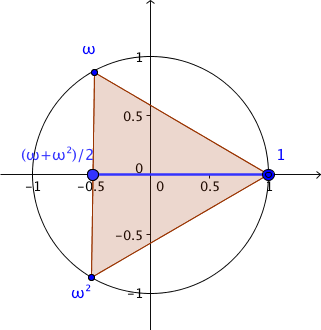
The first example is the simple average of a standard equilateral
triangle and its reverse, namely $\sfrac12(\chi_1+\chi_2)$. The
points are thus $(1,-\sfrac12,-\sfrac12)$; this is a degenerate
triangle of points with the second and third vertices coincident at
$-\sfrac12$. It is a digon with a double point at the left-hand end.
If we
separate the two triangles by making the standard one larger, say lying on a circle of
radius $\lambda>1$ then we get
$$\begin{eqnarray*}
\sfrac12(\lambda\chi_1+\chi_2)&=&
\sfrac12\left\{\lambda(1,-\sfrac12+\sfrac{\sqrt3}2\ii,-\sfrac12-\sfrac{\sqrt3}2\ii)
+(1,-\sfrac12-\sfrac{\sqrt3}2\ii,-\sfrac12+\sfrac{\sqrt3}2\ii)\right\}\\
&=&\sfrac12\left(\lambda+1,-\sfrac12(\lambda+1)+
\sfrac{\sqrt3}2(\lambda-1)\ii,-\sfrac12(\lambda+1)-\sfrac{\sqrt3}2(\lambda-1)\ii\right)
\end{eqnarray*}
$$
which shows the triangle is an isosceles one with height $\sfrac34(\lambda+1)$
lying along the real axis.
If we separate the two basic triangles $\chi_1$ and $\chi_2$ by
turning them in opposite directions by a turn $\ee^{\ii \alpha}$ (in
the attractive terminology of Frank Morley for complex numbers of modulus 1) to make
$$
\begin{eqnarray}
\sfrac12(\ee^{\ii \alpha}\chi_1+\ee^{-\ii \alpha}\chi_2)&=&
\sfrac12\left\{\ee^{\ii \alpha}(1,-\sfrac12+\sfrac{\sqrt3}2\ii,-\sfrac12-\sfrac{\sqrt3}2\ii)
+\ee^{-\ii \alpha}(1,-\sfrac12-\sfrac{\sqrt3}2\ii,-\sfrac12+\sfrac{\sqrt3}2\ii)\right\}\cr
&=& \left(\sfrac12(\ee^{\ii \alpha}+\ee^{-\ii \alpha}),
-\sfrac14(\ee^{\ii \alpha}+\ee^{-\ii \alpha})+
\sfrac{\sqrt3}4\ii(\ee^{\ii \alpha}-\ee^{-\ii \alpha})
,-\sfrac14(\ee^{\ii \alpha}+\ee^{-\ii \alpha})-
\sfrac{\sqrt3}4\ii(\ee^{\ii \alpha}-\ee^{-\ii \alpha})\right)\cr
&=&(\cos \alpha,
-\sfrac12\cos \alpha-\sfrac{\sqrt3}2\sin \alpha,
-\sfrac12\cos \alpha+\sfrac{\sqrt3}2\sin \alpha)
)
\end{eqnarray}
$$
then we have achieved a splitting of the double point at $-\sfrac12$
in $\sfrac12(\chi_1+\chi_2)$ but still have a degenerate triangle on
the real axis, with the second vertex at $z_1=-\sfrac12\cos
\alpha-\sfrac{\sqrt3}2\sin \alpha$ and the third symmetrically
placed about $-\frac12\cos\alpha$ at $z_2=-\sfrac12\cos
\alpha+\sfrac{\sqrt3}2\sin \alpha$.