IDL Tutorial for Astronomy 361
Prof. J. D. Monnier
2003Feb
This tutorial is meant to take approximately 2 hours and expose you to the basic functionality of IDL. After this tutorial (and with frequent consulation of idl help '?'), you should be able to effectively use IDL to analyze and present the data taken during subsequent experiments. There is no separate Worksheet to fill out, but rather the tutorial instructs you to create a 'JOURNAL' file of your IDL session and also asks you to create postscript plots at a number of junctures. Please name these files as instructed so I can review them later as part of the grading.
I have included links to other online IDL tutorials if you want to learn more; also, there are lessons in the IDL reference books in the 8th floor Dennison Computer Room.
After logging in as user astroclass (windows, lsa domain), I recommend you start IDL by clicking on the file: My Document\AY361\ay361 materials\idl_startup.pro (you should also be able to find IDL v5.2 under the Start menu).
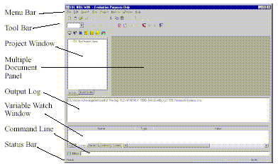
When you begin idl under Windows 2000, you will see the idl development environment (idlde):

The idlde environment allows you to look at local variables, edit procedures/scripts, inspect previous commands, and issue new commands.
To setup the environment properly, you need to compile thenrune the idl_startup.pro file mentioned previously. After opening this file in an IDL editor, you should be able to compile (using right mouse button or ctrl^F5) and to then run it (choose from right-button popup menu, or hit F5). This will set up your path and a few other things (for instance, you can browse the procedures of the Astronomy library in \My Documents\astron\contents).
Unlike in more structured programming languages (e.g., C++, Fortran), one does not have to explicitly define variables in IDL; rather, variables are defined implicitly through their use. For example,
IDL> a=1.0
IDL> i=1
IDL> help,a,i
A FLOAT = 1.00000
I INT = 1
You see that 'a' was declared as a float, while 'i' was declared as an integer. This information is also shown in the 'Variable Watch Window.' For more information on IDL data types, you can invoke IDL online help by typing a '?': try a search for 'data types.'
![]() IDL can also save all your interactive session by using the JOURNAL command, and this will part of your tutorial today instead of filling out a separate worksheet. Start the recording process by typing the following command.
IDL can also save all your interactive session by using the JOURNAL command, and this will part of your tutorial today instead of filling out a separate worksheet. Start the recording process by typing the following command.
IDL> journal,'YourName.Date.journal' ; e.g., journal, 'monnier.2003Mar19.journal'
When you exit IDL (or type 'journal' again with no filename), the reconding session will end. Please use JOURNAL to record your sessions for future reference. After typing a few commands, check that the file has been created in the proper place ('My Documents\AY361\ay361 users')
One can create arrays, 1-D or 2-D, easily as well.
IDL> x=[0,1,2,3,4,5]
IDL> y=fltarr(50) ; semicolon marks a comment line. use IDL> ? fltarr to see what this line does.
Try to understand what the following does using online help.
IDL> x= findgen(100)
IDL> y=10*randomn(seed,100)
IDL> plot,x,y,title='First plot',xtitle='X axis',ytitle='y axis label' ; IDL uses keywords to pass (often optional) information. Here we use the optional keyword XTITLE to label the x axis -- see online help for complete list of keywords
Note that a window (IDL 0) was created. You can create multiple plotting windows using IDL, and move between them easily. See online help for details on how to modify their default sizes, title bars, positions, etc.
IDL> window,0 & plot,x,y ; ampserand used to separate commands on the same line
IDL> window,1 & plot,x,y*y ; create new window and make a plot
IDL> wset, 0 & plot,x,x^2 ; go back to the first window and make a new plot
There are many ways to make a plot in IDL. Simple plots can be interactively created using LIVE_PLOT, or some version of LIVE_*. More generally, one makes a plot by opening a postscript device, issuing the plot commands, then closing the device -- thereby, creating a nice postscript file. See below:
IDL> set_plot,'ps' ;set postscript device
IDL> device, /landscape, filename = 'yourname.plot1.ps' ;e.g. monnier.plot1.ps ![]()
IDL> plot,x,y,xtitle='xlabel',ytitle='ylabel',title='Your Title Here'
IDL> device,/close ; close the postscript device... Did it create a good file??
IDL> set_plot,'win' ; for windows machine -- or set_plot,'x' ; for xwindows (linux/solaris)
What about Images? IDL is probably best used for doing image analysis. A quick way to create a dummy image in IDL is using the dist() function (IDL> ? dist):
IDL> im=dist(100,100)
and there are many built-in ways to display this data (use online help to see what each of these commands do):
IDL> surface,im
IDL> contour,im
IDL> contour,im,findgen(100)-50,findgen(100)-50,/c_ann,nlevel=20
IDL> shade_surf,im
IDL> tvscl,im
IDL> image_cont,im,/aspect ; using a / in front of a keyword is equivalent to setting it equal to 1, a useful shortcut for 'turning on' or enabling extra features in procedures/functions
IDL> show3, im
IDL> live_surface,im ;This program allows you to even rotate the surface around..
You can choose many color tables when viewing images. You can choose a palatte using 'xloadct' or:
IDL> loadct,3 ; you can see a list by just typing loadct w/o a number
Now replot images to see the new color table take effect:
IDL> image_cont,im,/asp
Try other color tables (I like 3 and 10 for general use) (if color does not work for you, you might try typing: IDL> device,decompose=0)
You can plot slices through the array by selecting certain rows/columns of the image:
IDL> plot,im[50,*] ; Note that [] brackets are prefered syntax for addressing array elements, while () paranthesis are meant for function calls
IDL> oplot,im[45,*],linestyle=2 ; the * wildcard lets you plot an entire row or column of an array
And it is easy to add a simple legend using the LEGEND command from the Astrolibrary:
IDL> legend,['row 50','row 45'],line=[0,2]
Since LEGEND is not a built-in IDL routine, you can not find help on it using the online help. However, you can use the following command to print out the routine's header.
IDL> doc_library,'legend'
You can access subarrays (a range of indices) easily using a colon
IDL> print,im[40:50,3]
IDL> image_cont,im[20:50,50:60],/aspect
Study the system variable !p.multi using the online help. This variable is used to make multiple plots on one page. Please use !p.multi to create one page of plots 3 across and 2 up/down. You should include plot, contour, and legend commands, and please label the axes.
![]() Save the multipanel plot as a postscript file: 'YourName.plot2.ps'
Save the multipanel plot as a postscript file: 'YourName.plot2.ps'
You can return to one plot per page by typing
IDL> !p.multi=0
One of the most important functions of a data analysis package is reading in data in variety of formats. IDL has some data formats built-in or programmed in the Astronomy library such as FITS. For instance, one can read in data from the Hubble Space Telescope using available libraries. Here, you can look at short exposure image of a binary star taken with the Keck Telescope:
IDL> image = readfits(dialog_pickfile()) ; Choose the file 'phiand.fits' in the 'ay361 materials' directory
Now, look at this image...
IDL> shade_surf,image ;loadct,3 produces a nice color table for shade_surf
IDL> tvscl,image
IDL> tv,hist_equal(image)
Try the following and see if you determine what the result means.
IDL> plot,image
You can see other data formats supported from the online help ('? read'), including GIF, JPEG, TIFF,. PNG, etc. etc. [Note that newer versions of IDL do not continue full support of GIF because of a licensing issues -- one can use the open format PNG.]
The smooth() command is helpful for visualizing images in some circumstances. Experiment with this function. What does the EDGE keyword do?
For the experiments in this class, the data is not stored in a 'standard' data format like FITS, but rather just recorded in ASCII format -- the numbers are just written in a text file. One can use a variety of methods to read ASCII data into variable arrays inside IDL. Lets try a few.
III. Reading in Data: Method 1: ascii_template()
IDL provides a GUI-based tool to help read in tabular data found in ascii files. The benefit of this method is that it is quick and easy -- however, it does not lend itself to scripting or automatic data processing.
First, look at the datafile in 'ay361 materials' directory called 'data1.txt' using the idle environment.
data1.txt:
Header Line 1: Sample data for AY361
-50.0000 -0.00264704
-49.0000 -0.0120685
-48.0000 -0.0188662
-47.0000 -0.0212358
-46.0000 -0.0183961
etc...
You see that the first line is text header followed by two columns of numbers. You can use ASCII_TEMPLATE() to define template to be used by the IDL program READ_ASCII() to painlessly absorb text data.
IDL> data_template = ascii_template() ; choose 'data1.txt'
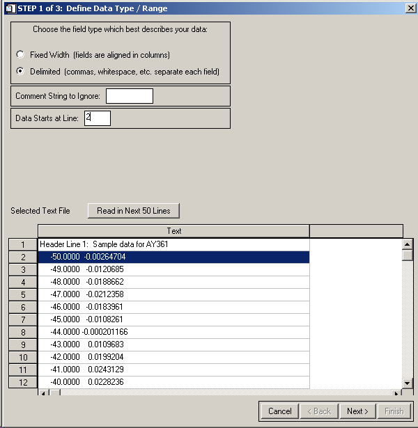
The bottom of the GUI shows you the file, while the top allows you to specify a few parameters. In this case we want to use 'Delimited' data and want to start reading data on line 2. It is common in ASCII data files to utilize a Comment String to make things more human-friendly -- you will see later that the Small Radio Telescope produces a data file which starts all comment lines with a '*' -- ASCII_TEMPLATE() provides an easy mechanism for ignoring these lines when reading in data.
OK, After setting things up as outlined above, hit Next>
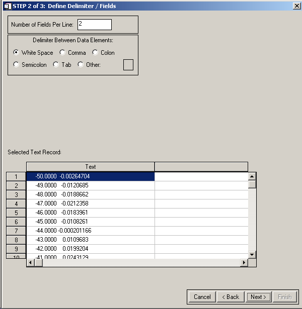
We are using White Space to delimit columns in this file and we see there are 2 fields per line. Set this up and hit Next>
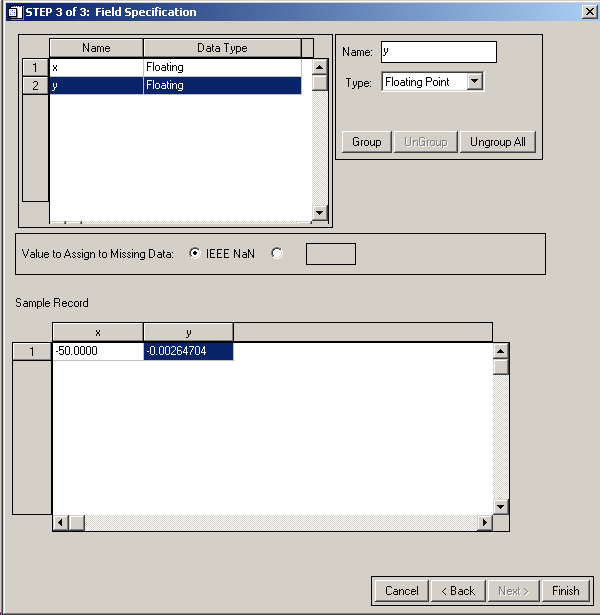
Click on the 2 different fields and change their names to 'x' and 'y'. Note that the program has automatically detected the data types of the fields (Floating Point), but allows you to specify something different. Hit Finish.
This has returned to IDL a structure (more info on -structures- below) containing the information on the ascii template. You can now attempt to read in the data and see if it correctly parsed the file:
IDL> data = read_ascii(template = data_template, header=header) ; you will have to choose data1.txt again.
IDL> help,data,/structure ; look at the data fields in the structure DATA (you can also use the Variable Watch Window to interrogate structures)
Those with little programming experience will recognize a 'structure' as a hybrid data type customizable for one's needs. In this case, DATA is a structure which contains a 100 element array called X and one called Y (you see how these names were defined in data_template using ascii_template(). Accessing the elements of a structure is simple by using a period '.' [Please read online help on structures for more info -- '? structures']
IDL> print,data.x
IDL> print,data.y[10:50]
IDL> plot,data.x,data.y,xtitle="X",ytitle="Y"
read_ascii() has a number of keywords (see online help). For instance, the lines which are skipped at the beginning of the file can accessed using the keyword HEADER.
IDL> print, header ; see the original read_ascii call above
![]() Please create a postscript plot of this line plot in 'YourName.plot3.ps'
Please create a postscript plot of this line plot in 'YourName.plot3.ps'
III. Reading in Data: Method 2: read_ascii() only
For very simple data files like 'data1.txt', it is very easy to skip the ascii_template() step entirely after a simple visual inspection of the datafile. Again -- read the online help for read_ascii() for more information.
IDL> data2= read_ascii(data_start = 1, delimiter = ' ', header=header2)
IDL> help,data2,/st ; keywords like /stucture can be abbreviated as long as the abbreviation is unique
You see that all the data is saved in an array called FIELD1. Also I see that the array is 7 x 100, which is obviously wrong. This is a bug in this version of read_ascii which counts the number of columns in the first line (header) instead of the first data line. Using IDL v5.4, FIELD1 has the correct dimensions (2,100). Despite this flaw, it still works enough to make a plot.
IDL> plot,data2.field1(0,*),data2.field1(1,*),xtitle="X",ytitle="Y",line=2
III. Reading in Data: Method 3: Using a script or procedure
One can also write custom functions or procedures to read in data files. This can be simpler in the long run if you have read in data over and over again and the data format does not change much. Look at the program called 'custom_data1.pro' in 'ay361 materials'. This program shows basic programming elements of IDL that you can use in your future data analysis programs. It can be utilized as follows:
IDL> filename = dialog_pickfile() ; choose data1.txt
IDL> custom_data1,filename,header,x,y
IDL> plot,x,y
Alternatively, one can return the data in a function call as a structure. See the file custom_data2.pro, which more closely replicates the usage behavior of read_ascii():
IDL> data3=custom_data2(filename,header=header)
IDL> help,data3,/st
IDL> plot,data3.x,data3.y,line=3
You just finished reading in 1-D data using different methods. In this section, we will assume the variables X & Y have been used to hold columns 1 and 2 respectively of data1.txt. Here we will just explore some of the features of 1-D plotting, including curve fitting, linestyles, plot symbols, legends, and error bars.
IDL> plot,x,y,xtitle="X",ytitle="Y",title="Test Plot", psym=4
Experiment with different plot symbols and linestyles-- see online help for the PLOT command.
You can easily overplot data onto an existing plot
IDL> oplot,x,y + 0.15, psym=2 ;use a different plot symbol or linestyle to tell the two datasets apart
The Astronomy Library has extra plot symbols you can use.
IDL> plotsym ; this will show you a list
IDL> plotsym,0,/fill ; this will set up plotsymbol 8 as a filled circle
IDL> plot,x,y,xtitle="X",ytitle="Y",title="Test Plot", psym=8
Usually, one has error bars associated with data. The Astronomy Library has a nice routine called ploterror (and oploterror) which allows you to plot error bars. See the following example:
IDL> err = replicate(.05,100) ; Create an array of error bars with value 0.05
IDL> ploterror, x,y,err,psym=8, xrange = [-10,10] ; XRANGE plots only a limited range along the x axis (similar for YRANGE)
IDL> plotsym,3,/fill ; setup a new plot (user defined) symbol
IDL> oploterror,x,y+.2,err,psym=8
Remember, that you can get the help on IDL routines using
IDL> doc_library,'ploterror' ; note that ploterror take the normal labeling keywords (xtitle,title, etc) as PLOT
For the rest of this part we will work with a reduced set of the data, and this will also introduce you to the useful IDL function called 'WHERE.'
IDL> index_array = where(x ge -10 and x le 10)
This will return the indices of the x-vector which satisfy the conditions inside the parentheses. 'ge' means 'greater than or equal to', 'le' means 'less than or equal to.' See online help for other conditional expressions ('? conditional'), such 'eq' = equals.
IDL> x0 = x[index_array]
IDL> y0 = y[index_array]
Inspect these variable arrays and plot the results. We now are only dealing with the part of the dataset near the origin. Lets try using a few of the built-in fitting routines in IDL.
IDL> result1= gaussfit(x0,y0,gauss_params)
IDL> poly_params=poly_fit(x0,y0,2,yfit)
Read the online help enough to understand what the parameters mean -- note how they have pretty different calls.
Now lets plot all of this and compare the fits:
IDL> plot,x0,y0,psym=4,title='Compare Fits',xtitle="X Axis",ytitle="Yaxis"
Now overplot (using OPLOT) result1 and yfit using different linestyles. Use the LEGEND procedure to label each curve. You see that this is quite a respectable plot, with labeled axes, a title, legend, etc. Please save a copy of this plot as 'YourName.plot4.ps'. ![]()
Analyzing 2-dimensional data is not that different in principle from analyzing 1-D data. Different routines are used to show contour plots and intensity images. When we map the sun using the UMRAO 26-m telescope, we will want to use IDL to graph and analyze the image. You saw some commands in the top section (surface, shade_surf, tvscl, etc); we work with these a little more here.
First load in a small image by restoring the variables in imagedata.sav
IDL> restore,'..\ay361 materials\imagedata.sav' ; or find it using restore,dialog_pickfile() if your path is not right
im: 21x21 image
x: coordinates of x axis
y: coordinates of y axis
info: a string variable containing a brief description of the above variables
As a test of data reading, try to use ascii_template() (GROUP features) and read_ascii() to read in the data from the ascii file imagedata.data. Compare the data in 'im' to the data you find with read_ascii() and make sure they are the same.
Now if just plot this image pixel for pixel onto the screen you will find the image awfully small.
IDL> tvscl,im ; remember to use loadct,3 and device,decompose=0 to see colors
The routine CONGRID() is used to copy a small array onto a much larger one, both with or without interpolation. See what happens:
IDL> tvscl,congrid(im,256,256)
IDL> tvscl,congrid(im,256,256,/cub)
IDL> big_image = congrid(im,256,256,/cub)
IDL> help,big_image
You were introduced to a number of routines above during the command-line exercises. Try making a contour plot of 'im' array, and label the axes with the values found in the arrays 'x','y'. Other routines to practice with: shade_surf, image_cont, others ?
You can also fit data using built-in fitting function
IDL> imfit=gauss2dfit(im,params) ;see online help for details of the call
You can compare the image with the fit:
IDL> contour,im,x,y,nlev=10,xtitle="Azimuth (deg)",ytitle="Elevation(deg)"
IDL> contour,imfit,x,y,/overplot, nlev=10,c_linestyle=2
IDL> legend,["Data","Gaussian Fit"],line=[0,2]
You can see the fit is very good. By the way, what were the parameters of the fit?
Another way to compare data is to make multiple plots on the screen using !p.multi. For instance, to make a 2x1 array of plots:
IDL> !p.multi=[0,3,1]
IDL> image_cont,im,/asp
IDL> legend,['Data']
IDL> image_cont,imfit,/asp
IDL> legend,['Gaussian Fit']
IDL> image_cont,im-imfit,/asp ; IDL adds/subtract arrays as easy as if scalars, if arrays are compatible
IDL> legend,['Residual Image']
Unfortunately, 'image_cont' is not a very flexible routine making axis-labelling problematic. One often has to write scripts to make publication quality plots for professional journals.
![]() The exercise (and postscript plot) of this section will be to draw 1-D scans through this image, one along the peak in x and one along the peak in y (curves should be labeled in the legend). Save as a single plot in the file 'YourName.plot5.ps' For extra credit, also overplot Gaussian fits to each scan and include the fitted parameters in the legend.
The exercise (and postscript plot) of this section will be to draw 1-D scans through this image, one along the peak in x and one along the peak in y (curves should be labeled in the legend). Save as a single plot in the file 'YourName.plot5.ps' For extra credit, also overplot Gaussian fits to each scan and include the fitted parameters in the legend.
Hint: You should be able to use contour and print statements to determine which pixel is the maximum. You could also experiment with the CURSOR command. Once you have found the peak pixel (x0,y0), you can plot the scans as shown in section II above.
Scripts allow you to automatically run a series of commands without having to type them in at the command line. This is particularly useful when executing a repetitive task, such as analyzing a number of data sets with the same procedure. Also, scripts are useful for making complicated plots since one generally wants to see the figure in the window before making a postscript figure. Here, we walk through a simple example of this.
For this exercise, you will be creating a file ("script") to run. If running on a windows machine, then you will be sharing the disk space with other users in AY361 and so you will have to name your files in a unique way. All your scripts should have names which obey the following style "YourName.script#.pro" so there are no conflicts (e.g., 'monnier.script1.pro'). You can save them in the 'ay361 users' directory if logged in as windows user astroclass.
So, open a new file using ctrl-N or using pulldown menu (File->New->Editor). Now you can type commands you would on the command line and these lines will be executed when the script is run. The only different rule is that this file must end with an 'end' statement.
As an example, lets put some of the commands from the previous exercises in a script:
in your new file:
; Test script written by -name- on -date- to do -what
; (header comments can be useful for future reference)
filename=dialog_pickfile()
custom_data1,filename,header,x,y
plot, x, y, xtitle="X Axis", ytitle="Y Axis",title="Plot made on:"+systime()
plotsym,0,/fill
oplot,x,y,psym=8
legend,['File: '+filename],box=0
end
![]() Now save this file as 'YourName.script1.pro' and then compile/run the program (remember to choose the datafile "data1.txt"). The easiest way to do this with the idlde gui is to right click in the editor window and choose 'Compile...' followed by 'Run ...'. After doing this, look at the plot that it made.
Now save this file as 'YourName.script1.pro' and then compile/run the program (remember to choose the datafile "data1.txt"). The easiest way to do this with the idlde gui is to right click in the editor window and choose 'Compile...' followed by 'Run ...'. After doing this, look at the plot that it made.
What about printing this? Using scripts, this is easy:
IDL> set_plot,'ps'
IDL> device,/landscape, filename = 'YourName.plot6.ps'![]()
IDL> .r filename.script ; or if you don't know the full path, etc., use the GUI to run script
IDL> device,/close
IDL> set_plot,'win' ; New plots will go to the screen as usual (with linux/solaris, type: set_plot,'x' instead)
You can now print your file using a postscript viewer like ghostview. On a unix machine, one can easily print this by spawning an lpr command:
[UNIX only:] IDL> spawn, 'lpr filename.ps' ; this will execute a unix shell command [not for windows]
| ? | Invoke IDL Online Help |
| <up arrow> | Scroll to previous commands |
| & | Separate multiple commands on same line |
| $ | Used to continue a command on the next line |
| ; | comment line |
| Printing | set_plot,'ps' & <plot commands> & device,/close & set_plot,'win' ; [or set_plot,'x'] |
| .run filename | Execute commands in the filename (run script!) |
| .continue | (or just '.c') allows a program/script to continue after a 'STOP' or break |
| save,/all,file='savesession.sav' | Save your IDL session to a file. Can start again next login using restore. |
| restore,'savession.sav' | Restores all files and compiled routines from previous session |