Krzysztof Fidkowski

mfoil: Matlab (and Python) airfoil analysis code similar to XFOIL
Back to top

mfoil

mfoil is a subsonic airfoil analysis code written as a single-file Matlab (and recently Python) class. It uses mostly the same physical models as XFOIL , with some differences in the coupled solver. As a Matlab code, it is slower than the Fortran code XFOIL and is not meant to be its replacement. Rather, it is an accessible code base for educational and research purposes. It is distributed under the open-source MIT license, which places virtually no restrictions on usage or modifications. You can download the latest version here:

Class file: mfoil.m (version 2021-10-13)

User interface: mfoilui.m (version 2021-10-13)

Documentation: mfoil.pdf (journal paper)

Python version: mfoil.py (version 2023-06-28)

Python version without LaTeX: mfoil_notex.py (version 2023-06-28)

User Interface

You can call the Matlab version of mfoil from scripts, functions, or the command line, as described below. Or, you can use the graphical user interface, mfoilui.m You can see "tooltip" help on using the GUI by hovering your mouse over various components, when the GUI is running.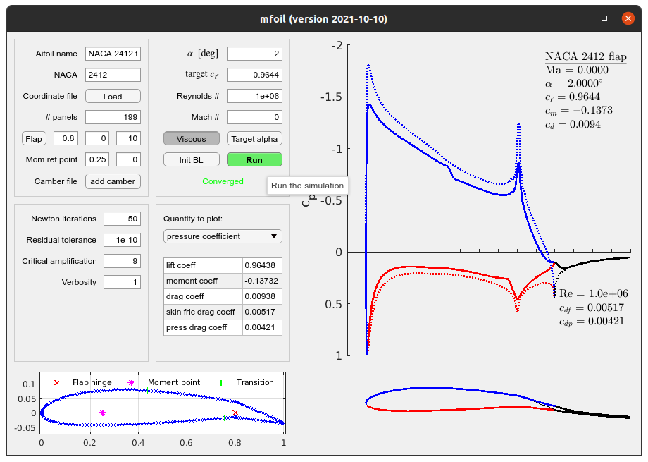 mfoil GUI

A tutorial video on using the GUI is provided below:

The Python version contains an example run setup in the main function at the end of the file. The capabilities are similar to that of the Matlab version.

Sample non-GUI usage

% viscous compressible flow over a NACA 2412 
% airfoil with a flap 

% create an airfoil class 
m = mfoil('naca','2412', 'npanel',199);

% introduce a flap 
m.geom_flap([0.85,0], 10);

% set operating conditions 
m.setoper('alpha',2,'Re',1e6, 'Ma',0.4);

% run the solver, plot the results (at right)  
m.solve

% for more boundary-layer plots  
m.plot_distributions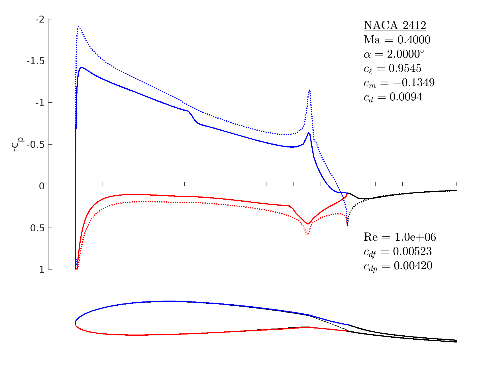

Note: all of the code examples here use the 'name',value syntax for passing arguments. Starting in R2021a, the name=value syntax is also supported, e.g.

 m = mfoil(naca='2412',
      npanel=199);

Capabilities

Coupled inviscid panel and viscous integral boundary layer equation solver
Kármán-Tsien compressibility correction
NACA 4 and 5-digit airfoils, or airfoils from provided coordinates
Basic geometry manipulation: flap, camber addition, derotation
Inviscid and viscous solutions at a prescribed angle of attack or lift coefficient
Viscous solutions at a given Reynolds number, including transition to turbulence
Boundary-layer initialization or reuse from previous solution
Access to all solution and post-processing variables
Plotting of results, including viscous distributions

Non-GUI Examples

Inviscid solution

% start with a 4-digit NACA airfoil 
m = mfoil('naca','2412', 'npanel',199);

% set angle of attack to 2 degrees 
m.setoper('alpha',2);

% run the solver, plot the results 
m.solve

% now set a constant lift coefficient 
m.setoper('cl',0.5);

% run the solver, plot the results 
m.solve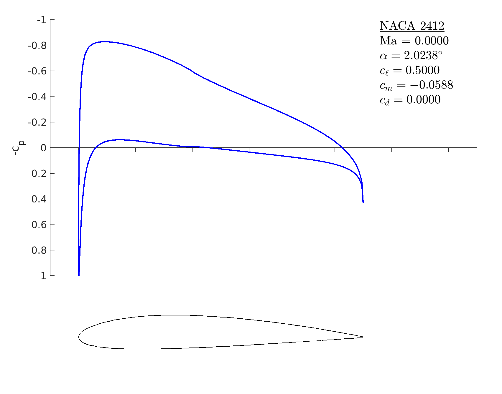

When an mfoil class is created, the default operating condition is zero angle of attack, inviscid, and incompressible. The results plot shows the pressure distribution on the airfoil (note the inverted axis) and displays the angle of attack and aerodynamic coefficients.

Viscous solution

% start with a 4-digit NACA airfoil 
m = mfoil('naca','2412', 'npanel',199);

% set angle of attack and Reynolds number  
m.setoper('alpha',2, 'Re',10^6);

% run the solver, plot the results 
m.solve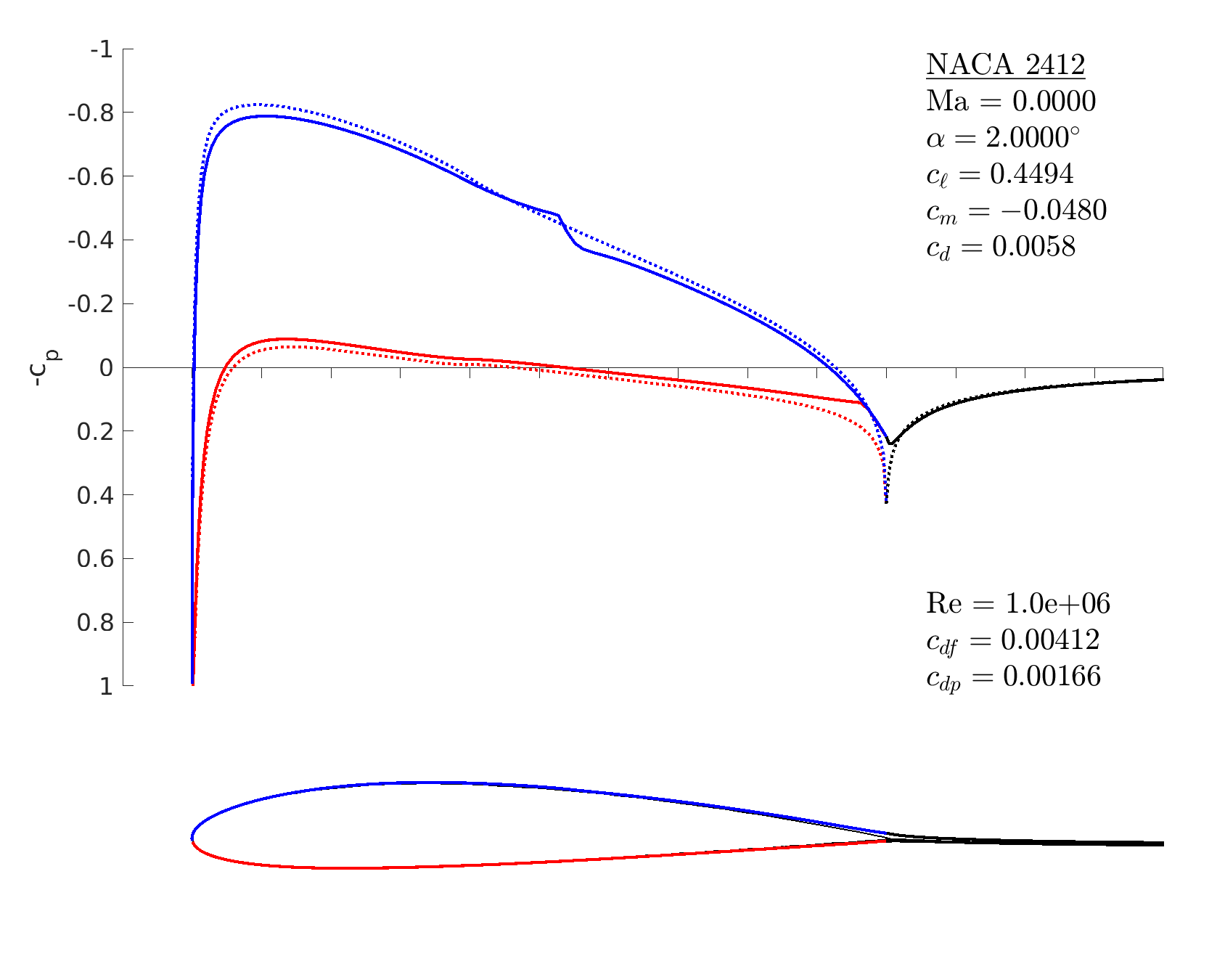

Setting the Reynolds number turns on the viscous mode. To go back to inviscid, specify visc=false when setting operating conditions, or just directly set


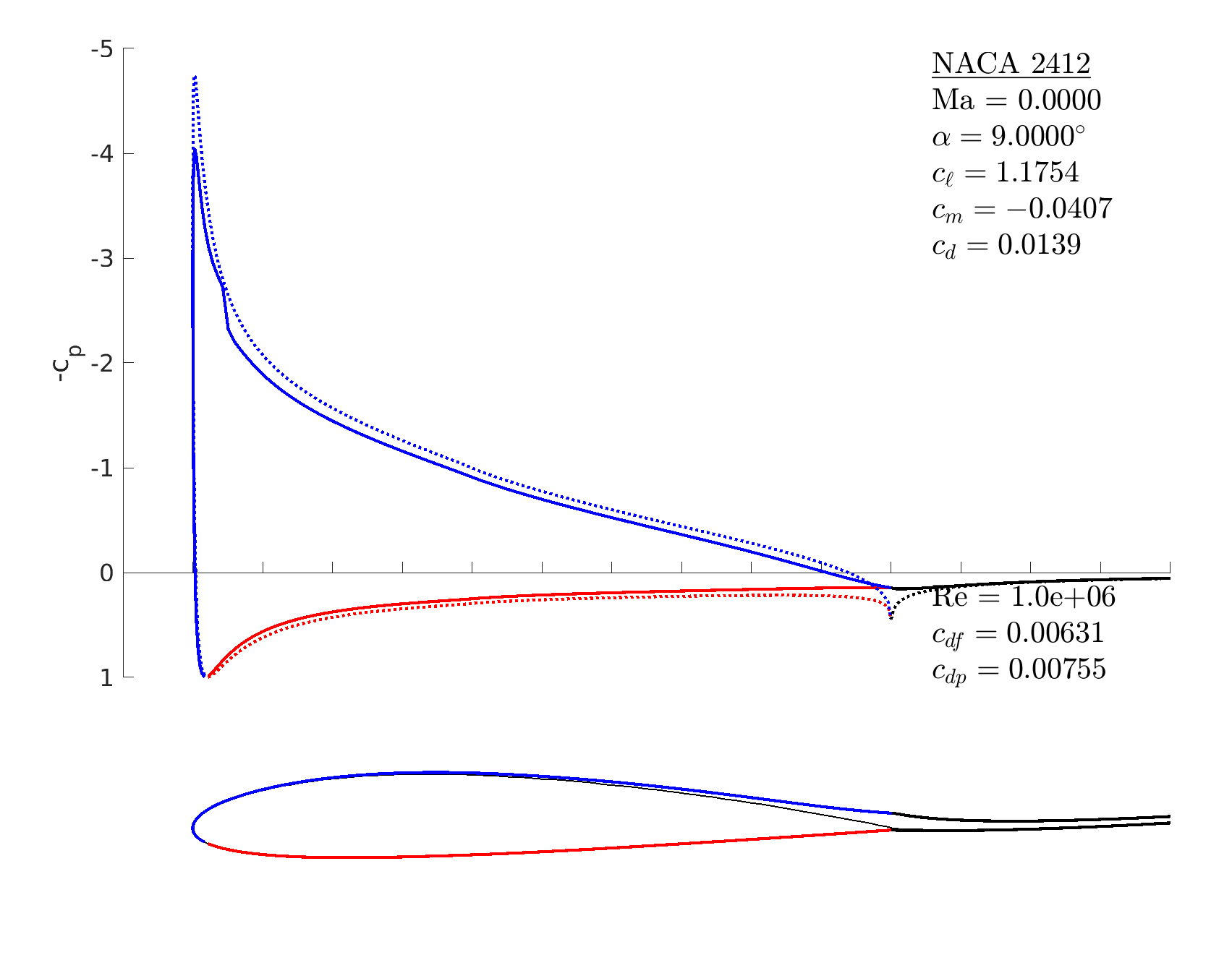
m.oper.viscous=false

. The viscous results plot now shows additional coefficients: the skin friction and pressure drag coefficients. The pressure coefficient plot distinguishes between upper (blue) and lower (red) surfaces, and the airfoil plot shows the boundary layer displacement thickness.

Coordinate import and flap

% import RAE 2822 airfoil coordinates 
X = load('rae.txt');

% make/panel an airfoil out of these coordinates  
m = mfoil('coords', X, 'npanel',199)

% introduce a flap at x=0.8, y=0, 10deg down  
m.geom_flap([0.8,0], 10)

% derotate: make the chord line horizontal 
m.geom_derotate
    
% set operating conditions 
m.setoper('alpha',1, 'Re',10^6);

% run the solver, plot the results 
m.solve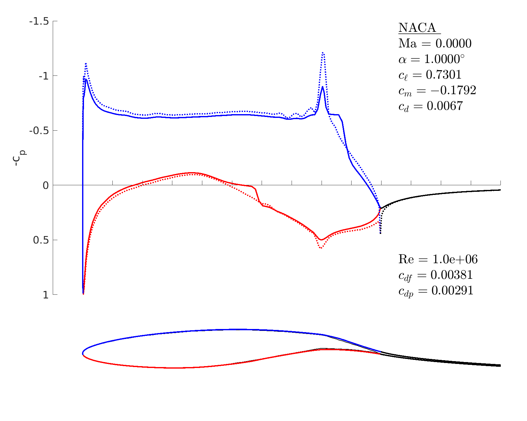

The coordinate file used in this example is rae.txt . It contains the (x,y) pairs of points on the airfoil, starting/ending at the trailing edge (there is a gap). Note, if there is no gap, the first/last points are duplicated. The points can be ordered clockwise or counterclockwise.

Modifying the camber

% start with a symmetric NACA airfoil 
m = mfoil('naca','0008', 'npanel',199);

% make points for a camber line addition 
x = linspace(0,1,101);
z = 0.03*sin(2*pi*x);

% add the camber to the airfoil 
m.geom_addcamber([x;z]);

% set operating conditions 
m.setoper('alpha',2, 'Re',10^6)

% run the solver, plot the results 
m.solve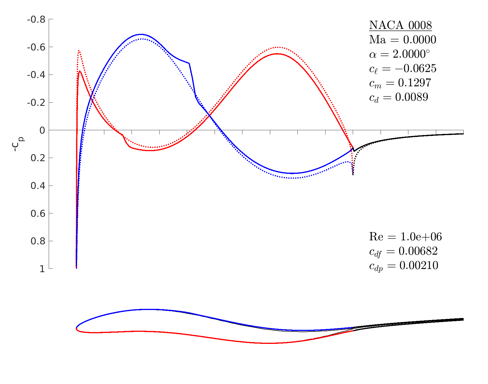

Calling m.geom_addcamber changes the vertical (z) position of each point on the airfoil surface by an interpolation of the provided (x,z) camberline coordinates. So if the airfoil already has camber, the camberline is incremented (not replaced).

Compressible flow

% start with a 5-digit NACA airfoil 
m = mfoil('naca','23012', 'npanel',199);

% set a nonzero Mach number  
m.setoper('alpha',2, 'Ma',0.6)

% run the solver, plot the results 
m.solve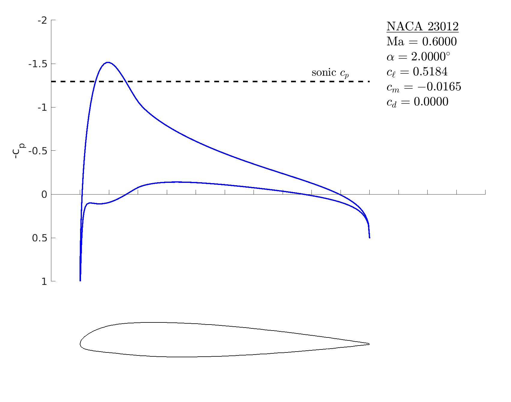

Setting a nonzero Mach number turns on the compressibility correction, which loses accuracy at higher Mach numbers and is not valid once shocks are present. The results plot will show a sonic pressure coefficient line (dashed) if this value is in the range of the current axes. If the pressure coefficient somewhere on the airfoil crosses this line, this indicates the onset of supersonic flow and the results should not be trusted.

Convergence issues

% start with a 4-digit NACA airfoil 
m = mfoil('naca','2412', 'npanel',199);

% set a difficult operating condition  
m.setoper('alpha',9, 'Re',10^6);

% try the solver ... does not converge (see right)  
m.solve

% set a related easier operating condition  
m.setoper('alpha',5, 'Re',10^6);

% run the solver  
m.solve

% turn off BL initialization 
m.oper.initbl = false;

% set the difficult operating condition  
m.setoper('alpha',9, 'Re',10^6);

% run the solver: now converges (right, bottom) 
m.solve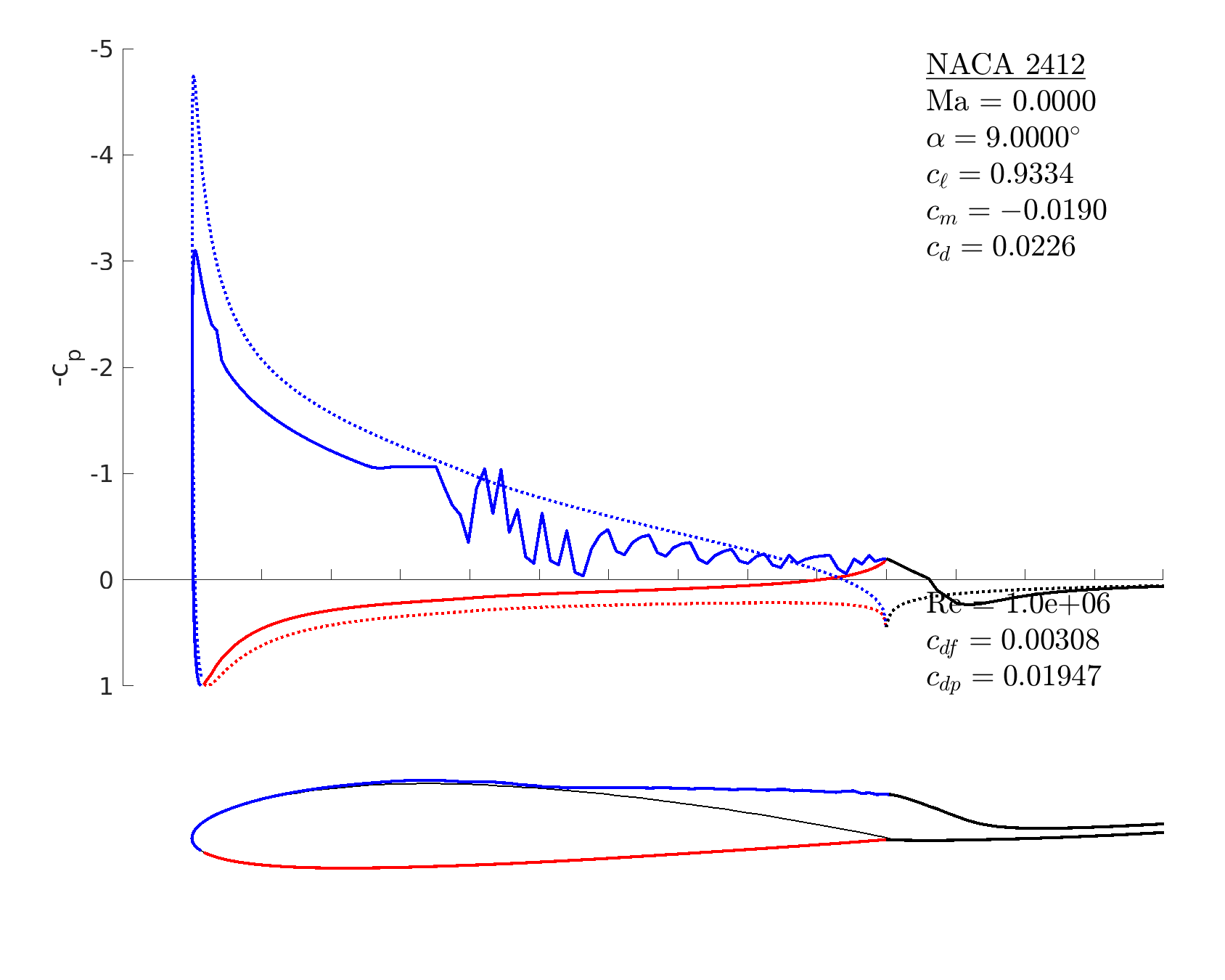

The coupled inviscid-viscous solver uses a Newton-Raphson method that can fail when the initial guess, which comes from an uncoupled initialization, is not very good. This generally happens at high angles of attack or low Reynolds numbers, when the flow is in danger of separation. Using a converged solution that is close to the desired one (e.g. at a lower angle of attack) can help, as shown above. To enable solution reuse, turn off boundary-layer state initialization, m.oper.initbl = false.

Changing settings

% ask for more verbose output during a run: 0 = quiet, 3 = verbose 
m.param.verb = 3;

% allow for more Newton iterations: default is 50 
m.param.niglob = 100;

% make Newton convergence tolerance less strict: default is 1e-10 
m.param.rtol = 1e-8;

% decrease critical amplification factor for transition: default is 9 
m.param.ncrit = 8;

% rebuild the wake during a viscous solution when alpha changes: default is false 
m.param.redowake = true; 

% destroy the mfoil class m 
clear m;

The m.param structure includes other parameters that can be adjusted directly. These include thermodynamics and viscous closure parameters. For more detailed descriptions, see the comments in the code.

Plotting

% NACA airfoil: set operating conditions and run the solver 
m = mfoil('naca','2412', 'npanel',199);
m.setoper('alpha',3, 'Re',1e6);
m.solve

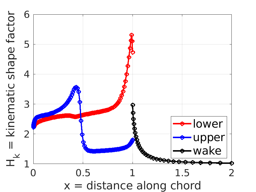
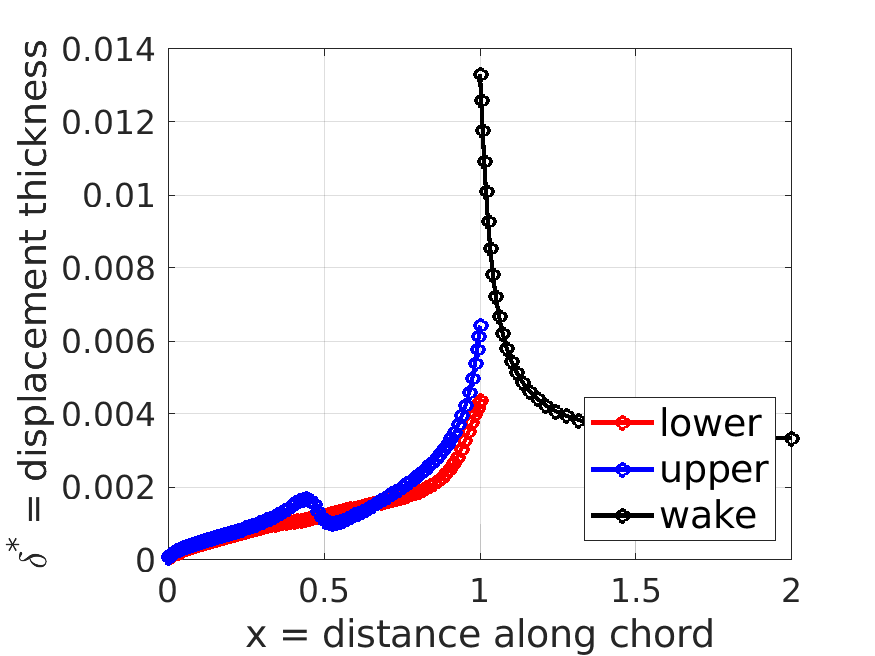
% make multiple figures of viscous variable distributions 
m.plot_distributions;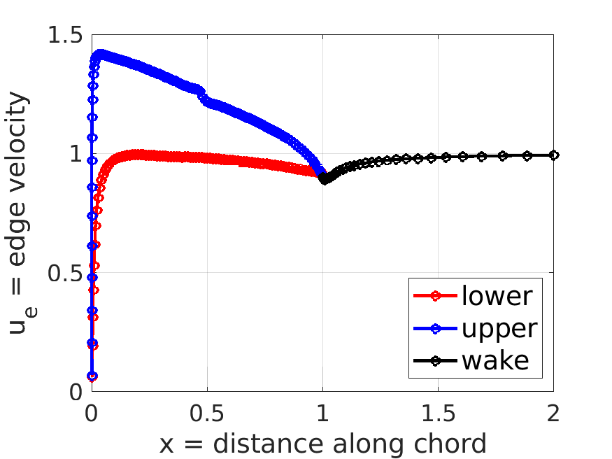

% plot the sreamlines over a default range 
m.plot_stream([],101);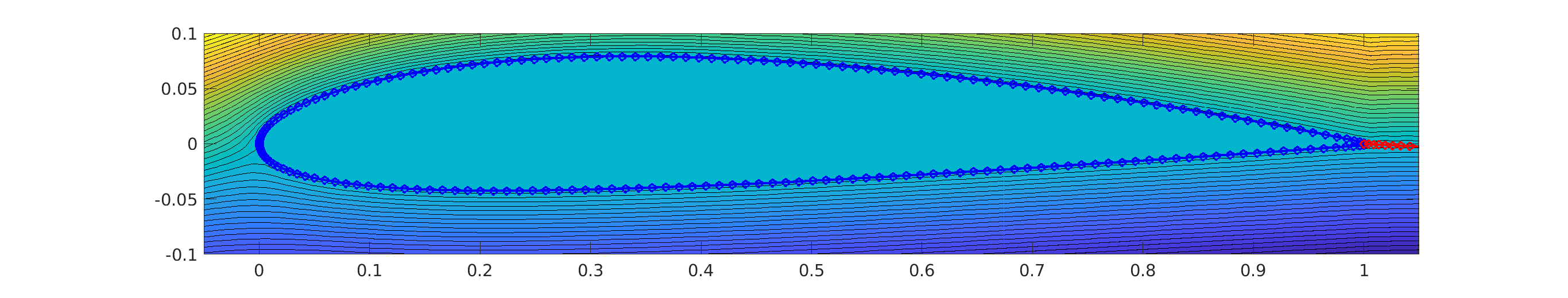

% plot streamlines near the trailing edge [xmin, xmax, zmin, zmax] 
m.plot_stream([.98, 1.03,-.004,.005],201);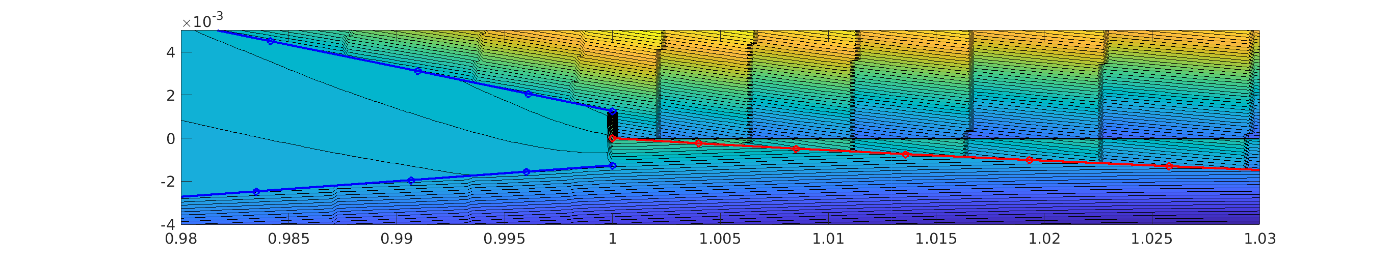

Note, the concentrated lines emanating perpendicularly from the panels are branch cuts of the viscous source panel streamfunctions. The dark horizontal line is the branch cut of the inviscid-solution source panel across the trailing-edge gap.

% plot velocity vectors 
m.plot_stream([-.1, 1.1,-.2,.2],51);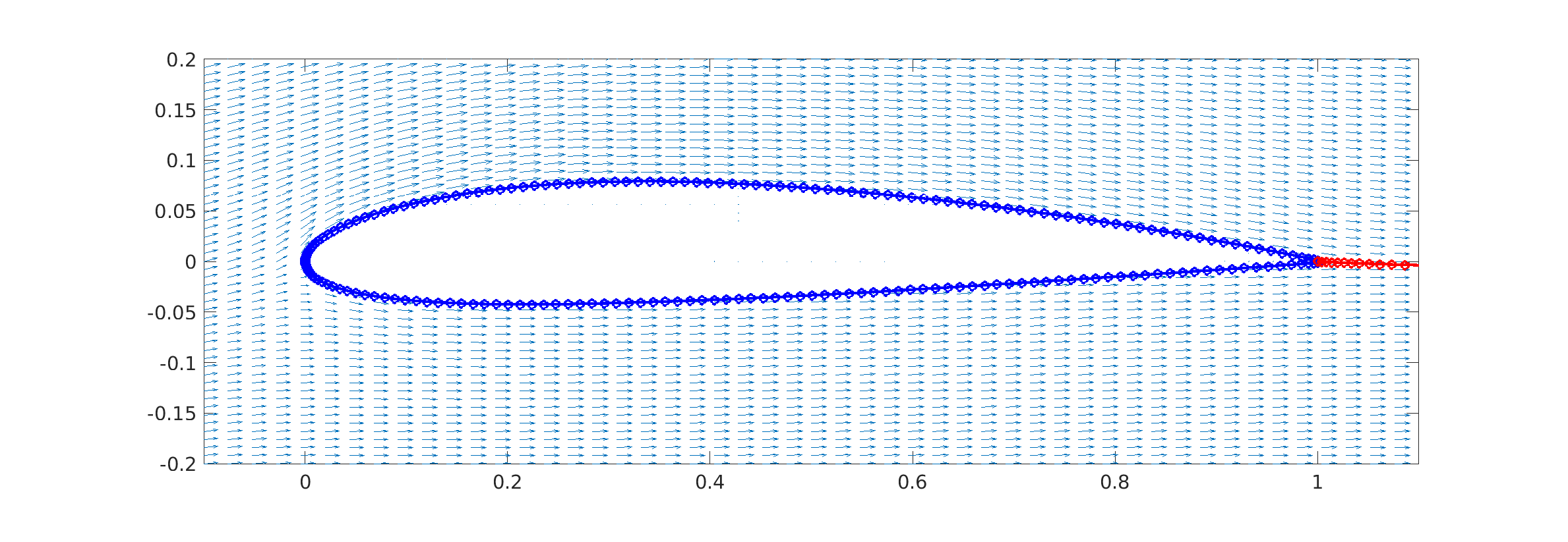

Access to data

% post-processed quantities are in m.post; these include 
m.post.cp;       % cp distribution 
m.post.cpi;      % inviscid cp distribution 
m.post.cl;       % lift coefficient 
m.post.cm;       % moment coefficient 
m.post.cdpi;     % near-field pressure drag coefficient 
m.post.cd;       % total drag coefficient 
m.post.cdf;      % skin friction drag coefficient 
m.post.cdp;      % pressure drag coefficient 

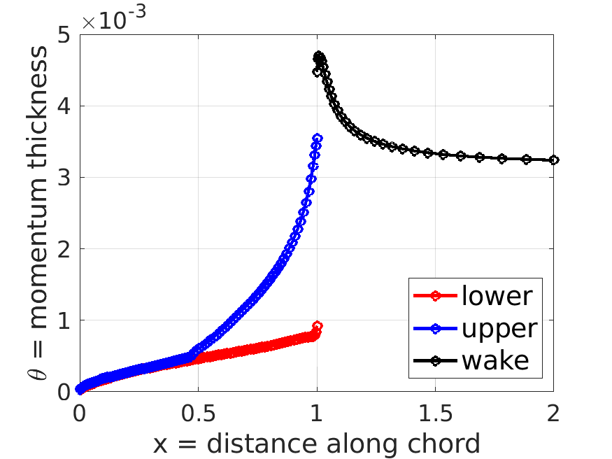
m.post.th;       % theta = momentum thickness distribution 
m.post.ds;       % delta* = displacement thickness distribution 
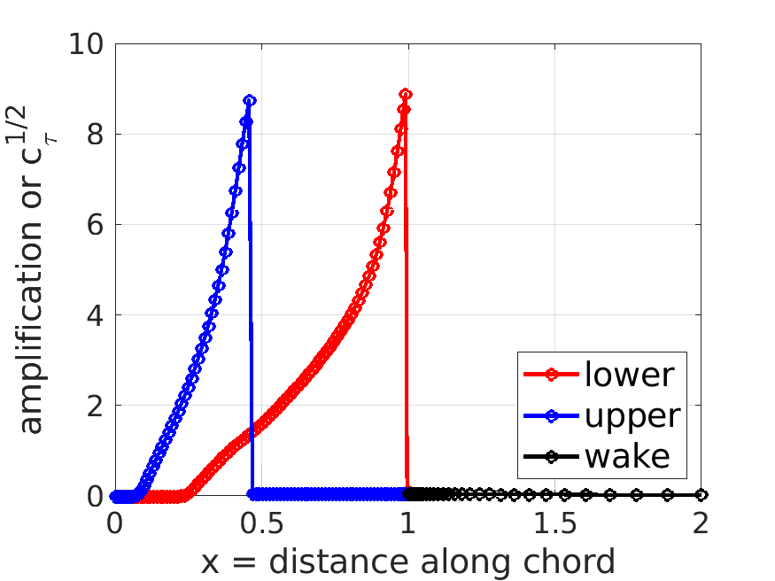
m.post.sa;       % amplification factor/shear lag coeff distribution 
m.post.ue;       % edge velocity (compressible) distribution 
m.post.uei;      % inviscid edge velocity (compressible) distribution 
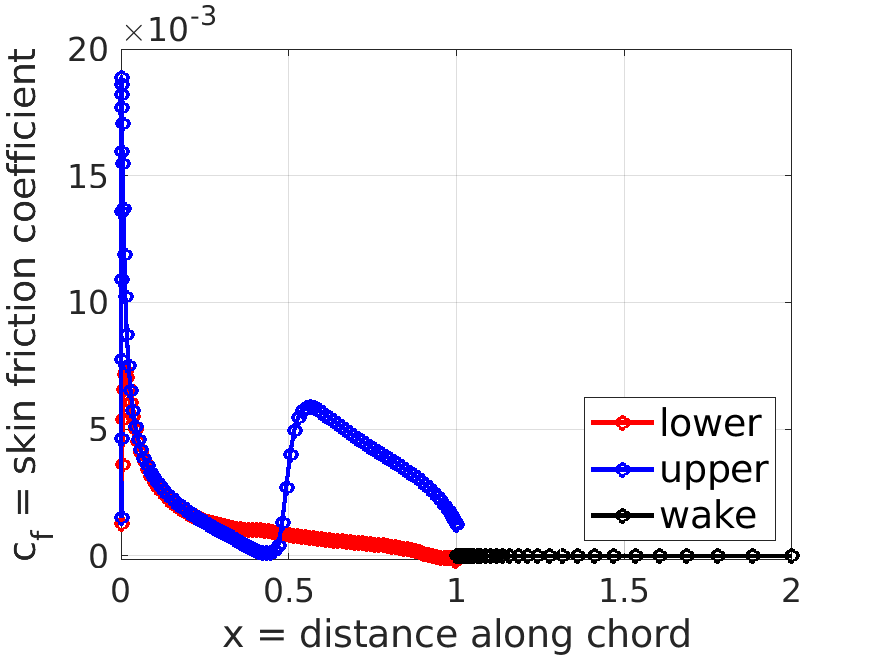
m.post.cf;       % skin friction distribution 
m.post.Ret;      % Re_theta distribution 
m.post.Hk;       % kinematic shape factor distribution 

% the inviscid solution (vorticity distribution) is stored in m.isol 
m.isol.AIC;      % aero influence coeff matrix 
m.isol.gamref;   % 0,90-deg alpha vortex strengths at airfoil nodes 
m.isol.gam;      % vortex strengths at airfoil nodes (for current alpha) 
m.isol.xi;       % distance from the stagnation at all points 


% the viscous BL solution, residual, and Jacobian are stored in m.glob 
m.glob.U;        % primary states (th,ds,sa,ue) [4 x Nsys] 
m.glob.dU;       % primary state update 
m.glob.dalpha;   % angle of attack update 
m.glob.R;        % residuals [3*Nsys x 1] 
m.glob.R_U;      % residual Jacobian w.r.t. primary states 
m.glob.R_x;      % residual Jacobian w.r.t. xi (s-values) [3*Nsys x Nsys]

Krzysztof J. Fidkowski

mfoil

User Interface

Sample non-GUI usage

Capabilities

Non-GUI Examples