Some brief background: RUV is distributed as a collection of R packages. The packages are: ruv, ruv.extras, ruv.htmllatex, and several data packages. The ruv package contains the core statistical routines. The ruv.extras package includes routines for making plots and example scripts (including ruv_starter_analysis). The ruv.htmllatex package is a dependency of ruv.extras that generates html.
The core statistical routines provided by the ruv package are RUV-2, RUV-4, RUV-inv, RUV-rinv, and a few others. These routines are meant for use by you, the end-user, but they are not the focus of this how-to. For more information on these routines, please consult the standard R package documentation. For more information on the statistical methodology behind these routines, please consult the references at http://www-personal.umich.edu/~johanngb/ruv.
IMPORTANT: The analyses performed by ruv_starter_analysis should not be considered complete, final analyses, but rather as a starting point for further investigation. Moreover, the ruv_starter_analysis script should not be considered part of the "core" of RUV. It may be more properly thought of as a demo of what one can do with the ruv package (albeit an elaborate and particularly useful demo). Thus, you are encouraged to modify this script to fit your own individual needs (see "Going Further" below). Moreover, in future releases of RUV, this script may be modified, perhaps in a way that is not backwards-compatible, perhaps beyond recognition, and may even be omitted entirely. For this reason, ruv.extras is not on CRAN.
ruv_starter_analysis(Y, X, ctl)All that is absolutely required is a data matrix Y, a factor of interest X, and a set of control features (control genes). For example, you could try running:
library(ruv.extras)
library(ruv.data.gender.sm)
data(gender.sm)
ruv_starter_analysis(gender.sm$Y, gender.sm$X, gender.sm$hkctl)
However, for our first example we will make use of a few addional features:
library(ruv.extras)
library(ruv.data.gender.sm)
data(gender.sm)
ruv_starter_analysis(gender.sm$Y, gender.sm$X, gender.sm$hkctl,
                     pctl=gender.sm$pctl, geneinfo=gender.sm$geneinfo, kset=c(1,5,10),
                     outdir="gender1", webtitle="Gender Example 1")
Here, pctl is a set of positive controls, geneinfo is a matrix including gene names and chromosome numbers, kset is a set of the values of K that we wish to consider, outdir is the directory where the web page will be written, and webtitle is the html title. The webpage output by running the above commands looks like this: Gender Example 1
As you can see, the web page is divided up into 9 sections: General Info, Unadjusted, RUV-2 Combined Analyses, RUV-2 Individual Analyses, RUV-4 Combined Analyses, RUV-4 Individual Analyses, RUV-inv, RUV-rinv, and Projection Plot Table. Each of these sections can be hidden / unhidden by clicking on the section title heading. This makes navigating the web page a bit easier (since it can be quite big), and also allows you to more easily compare different analyses (e.g. by hiding the RUV-2 and RUV-4 analyses, the Unadjusted and RUV-inv analyses will be next to each other). Individual subsections (RLE plots, p-value plots, etc.) can be hidden as well.
Now let's go through and see what each of these sections has to offer.
m = 84, n = 12600, n_c = 799
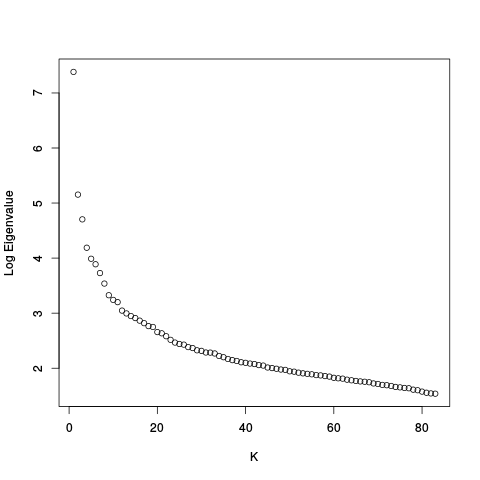
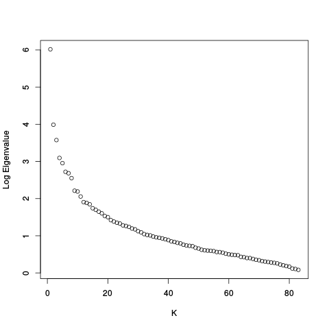
After this there are scree plots:
| Y | Y_c |
|
|
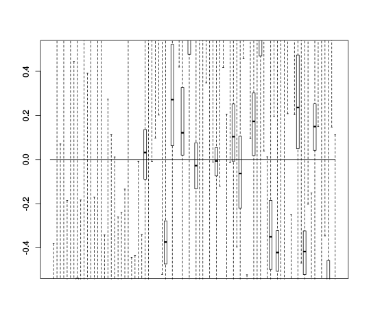
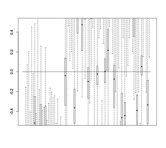
After the Scree plots come RLE plots:
| Y | Y_c |
 |
 |
After the RLE plots comes a canonical correlation plot.
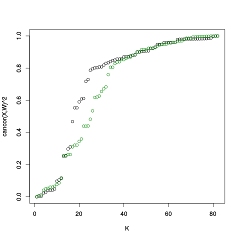 |
After the canonical correlation plot comes a table of principal component plots. An SVD is taken of Y (and also Y_c), and the left singular vectors are referred to as factors. We denote this matrix of factors by W_all (or W_ctl in the case of Y_c). In these plots, we plot one factor against another. This is helpful for seeing if there are any clusters or other interesting variation in the data, and also whether the variation in the control features (genes) is representative of the variation in the entire dataset. The factors of Y are plotted on the right, and the factors of Y_c are plotted on the left.
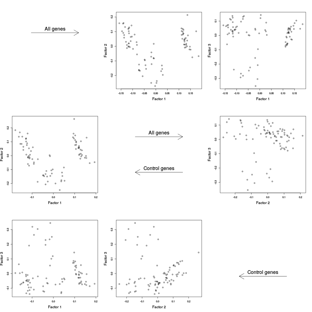 |
Finally, the General Info section concludes with a table of alpha plots. These are similar to the PC plots, except that instead of plotting the factors (columns of W) against one another, we plot the rows of alpha against one another. Here, alpha is equal to W_all'Y in the plots on the right, and W_ctl' Y in the plots on the left.
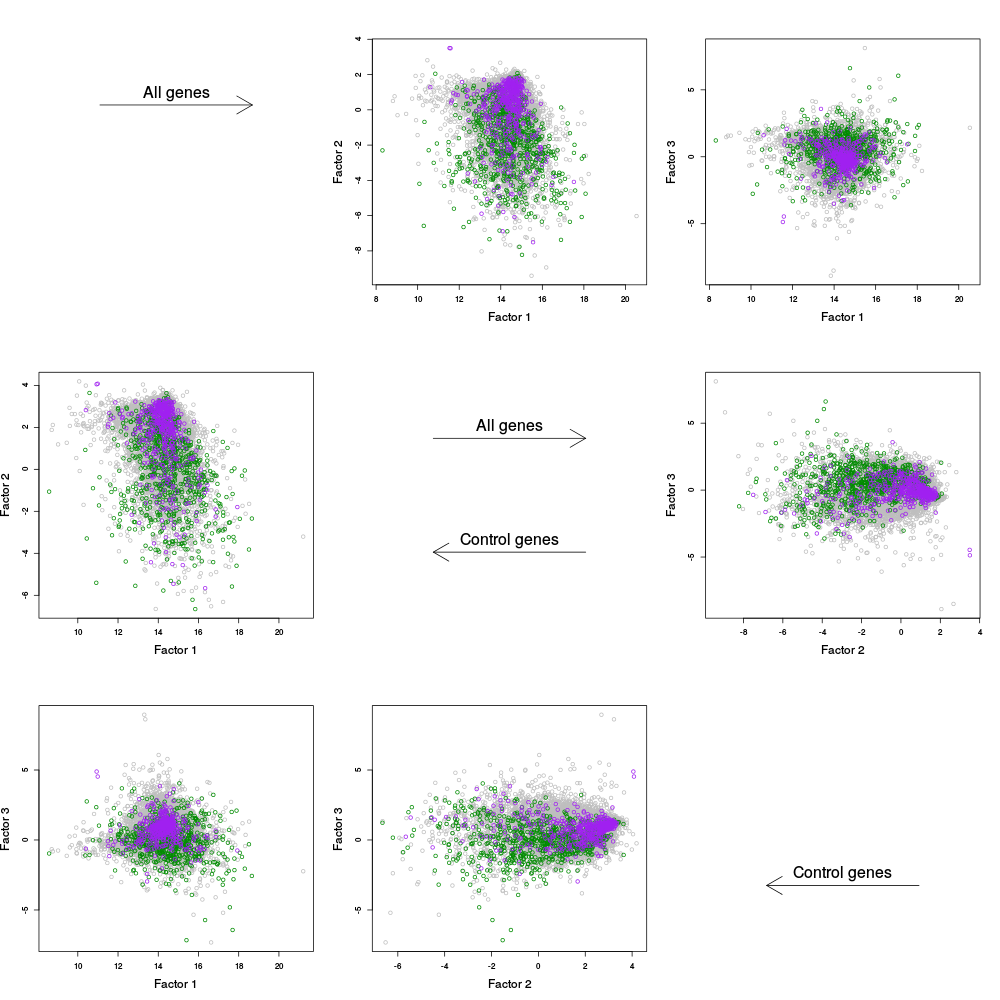 |
The first plots are RLE plots. These plots differ from the RLE plots in the General Info section only in that here, the data has first been adjusted by known covariates Z, if in fact a Z matrix has been supplied.
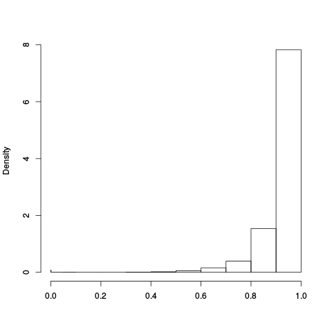
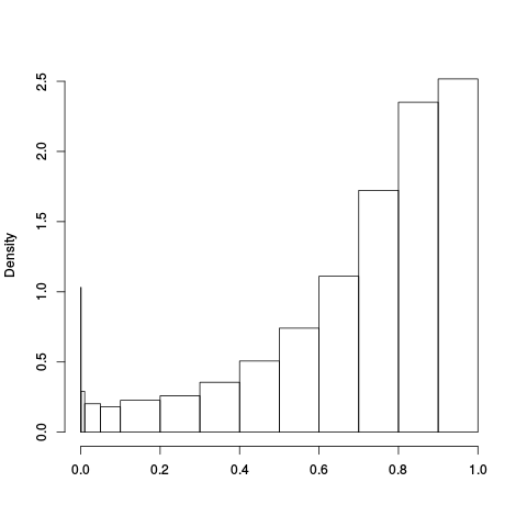
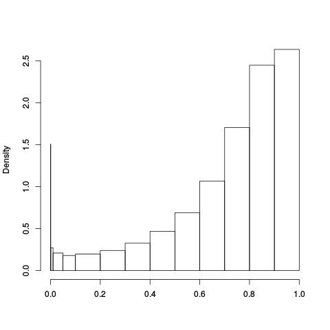
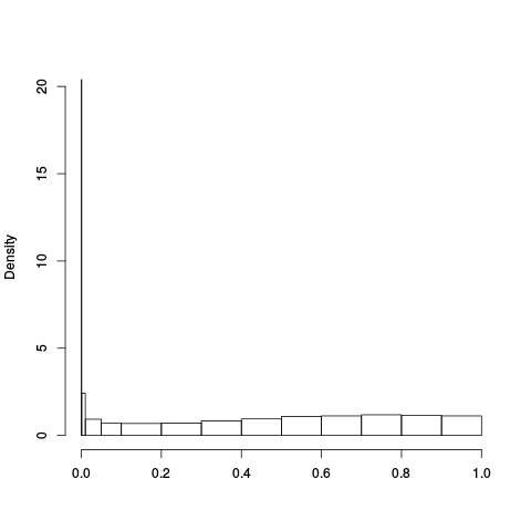
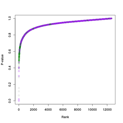
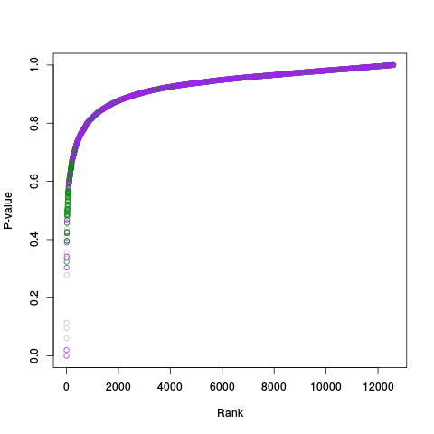
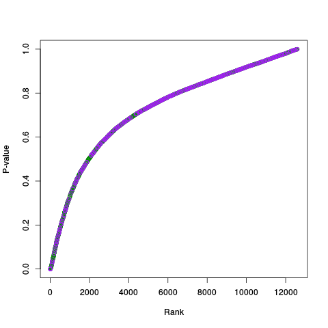
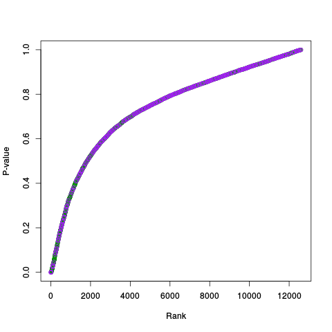
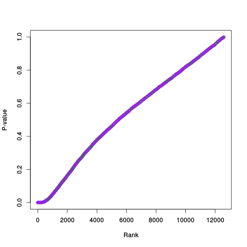
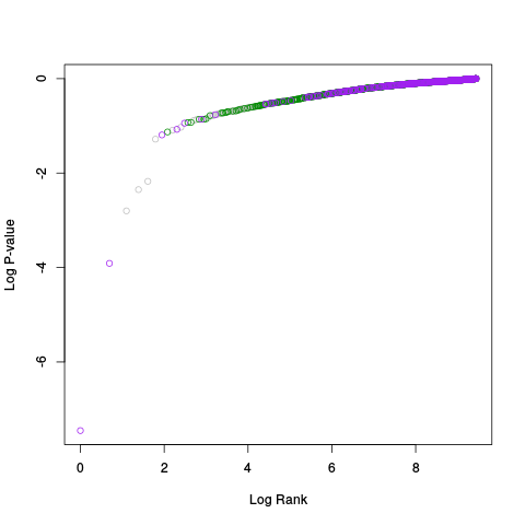
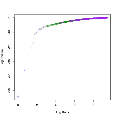
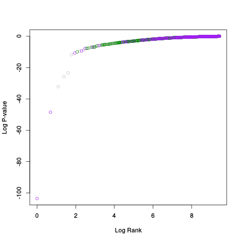
Following the RLE plots are a table of p-value plots:
| standard | ebayes | rsvar | rsvar ebayes | evar |
 |
 |
 |
 |
 |
 |
 |
 |
 |
 |
 |
 |
 |
 |
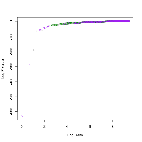 |
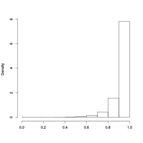
A second table of p-value plots is then shown, in which only p-values of the negative controls are plotted. Ideally, the histograms will be flat, and the qq plots will be straight lines. The extent to which the histograms are not flat and the extent to which the qq plots are not straight lines give us some indication of how much unwanted variation is present in the data.
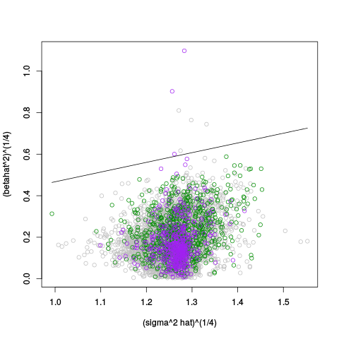
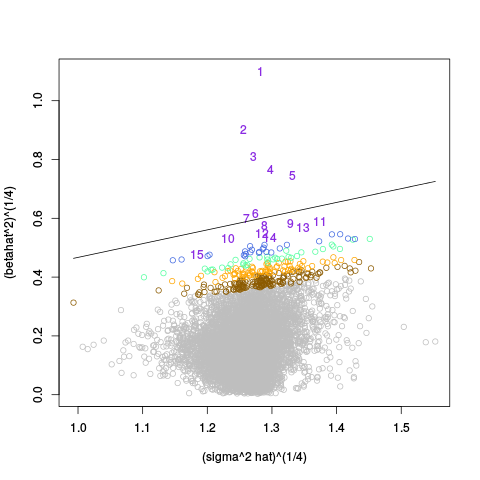
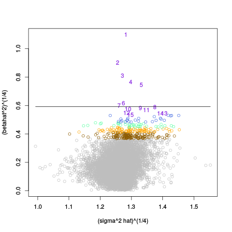
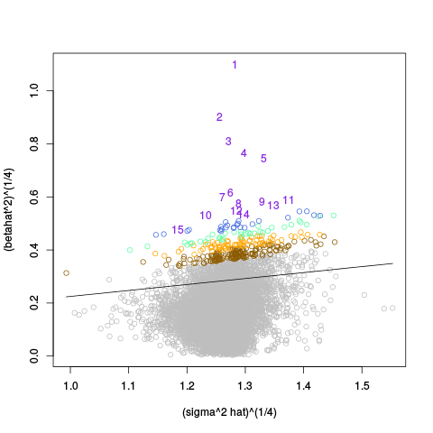
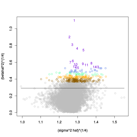
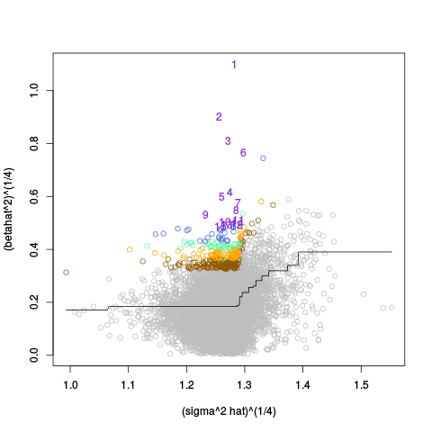
Following the p-value plots are variance plots.
| Standard Coloring | standard | ebayes | rsvar | rsvar ebayes | evar |
 |
 |
 |
 |
 |
 |
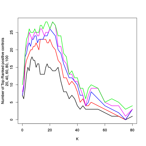
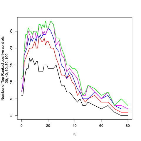
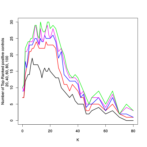
After the variance plots are a set of tables showing how many positive controls are found in the top N most highly-ranked features (genes). By default, values of N = 20, 40, 60, 80, and 100 are shown, but this can be changed using the topcount_threshold variable. (Note: If no positive controls are specified, this section will not exist.)
| standard | ebayes | rsvar | rsvar ebayes | evar | ||||||||||||||||||||||||||||||||||||||||||||||||||
|
|
|
|
|
Finally, the Unadjusted section concludes with tables of the top N most highly ranked features (genes). By default N is 40, but this can be changed using the topN variable. Tables are provided for each of the 5 methods of computing p-values.
If you click on an entry of the table, you will get the results of a google search for that entry. This is useful for quickly googling the genes.
| standard | ebayes | rsvar | rsvar ebayes | evar |
 |
 |
 |
 |
 |
The second table of plots (not shown) includes RLE plots, a projection plot, and an extensive variety of p-value plots for each value of K. These plots are all duplicated in the RUV-2 Individual Analyses section (below), but are included here in one giant table so that an easy comparison between different values of K can be made. It will be very helpful to hide various rows / columns when viewing this table.
| Standard Coloring | standard | ebayes | rsvar | rsvar ebayes | evar |
 |
 |
 |
 |
 |
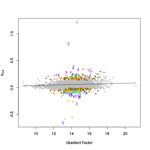 |
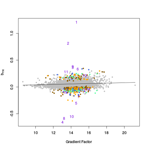
TODO: Describe Projection plot table
Y |
The data. A m by n matrix, where m is the number of samples and n is the number of features. |
X |
The factor of interest. A m by 1 matrix, where m is the number of samples. |
ctl |
The negative controls. A logical vector of length n. |
Z |
Any additional covariates to include in the model. Either a m by q matrix of covariates, or simply 1 (the default) for an intercept term. |
eta |
Gene-wise (as oposed to sample-wise) covariates. These covariates are adjusted for by RUV-1 before any further analysis proceeds. A matrix with n columns. |
pctl |
Positive controls. A logical vector of length n. |
genecoloring |
A vector of length n. The colors to use when plotting genes. |
samplecoloring |
A vector of length m. The colors to use when plotting samples. |
genetexts |
A vector of length n. Any text to be used in place of symbols, when plotting genes. Elements that are NA are plotted as symbols. |
sampletexts |
A vector of length m. Any text to be used in place of symbols, when plotting samples. Elements that are NA are plotted as symbols. |
genesymbols |
A vector of length n. The plot symbols to use when plotting genes. |
samplesymbols |
A vector of length m. The plot symbols to use when plotting symbols. |
geneinfo |
A matrix with n rows. Each column should contain some information about the genes (such as their names) for use in tables. |
rankbybeta |
Should the analysis include a ranking of the features based on the absolue value of estimated effect size (betahat)? |
topN |
The number of top-ranked genes to include in tables. |
topcount_thresholds |
The thresholds to use when counting the number of top-ranked positive controls. |
rankset |
The genes to be considered when determining which are top-ranked. A logical vector. NULL implies all genes. |
kset |
Which values of K should be considered. |
factorset |
Which factors should be included in the projection plot table. |
bin |
The bin size in the method of empirical variances. |
do_general |
Should the "general" analysis be performed? |
do_unadjusted |
Should the "unadjusted" analysis be performed? |
do_ruv2 |
Should the RUV-2 analysis be performed? |
do_ruv4 |
Should the RUV-4 analysis be performed? |
do_ruvinv |
Should the RUV-inv analysis be performed? |
do_ruvrinv |
Should the RUV-rinv analysis be performed? |
do_pptable |
Should the factor projection plot table be created? |
outdir |
Directory where the web page should be written. |
initialize_collapsed |
Should the web page be created so that only headers are shown, and must be manually expanded? |
webtitle |
The title of the web page. |
inputcheck |
Perform a basic sanity check on the inputs, and issue a warning if there is a problem. |
verbose |
Verbose output. |
A few of these arguments warrant further comment.
First note that X must consist of only a single column. Although RUV-2, RUV-4, etc. support an X with more than one column, ruv_starter_analysis does not. This is because many of the plots (e.g. p-value histograms, projection plots) only make sense in the context of a single-column X. If you have several factors of interest, the easiest way to handle this situation is to run ruv_starter_analysis several times, each time setting X to be just one of the factors of interest. If desired, the remaining factors of interest can be included in the model by including them in the Z matrix.
The do_unadjusted, do_ruv2, do_ruv4, do_ruvinv, do_ruvrinv, and do_pptable arguments can be set to FALSE in order to omit these sections of the analysis and speed up execution.
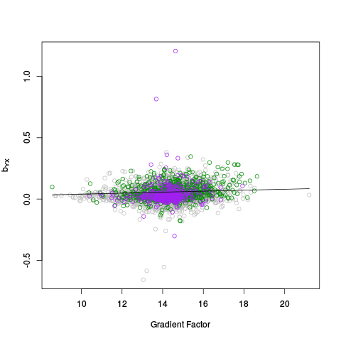
The genecoloring and samplecoloring arguments can be used to specify the colors used in the plots. If there are any NAs in the coloring vector, those samples / features will be plotted in light gray. If a coloring vector is not specified at all, by default, all features are plotted in light gray except for negative controls, which are plotted in green, and positive controls (if they are given), which are plotted in purple. NOTE: The plots are done in a special way, so that points of "rare" colors are plotted last, to ensure they are visible. So, for example, if there are 10,000 gray points, 1,000 green points, and 100 purple points, all 10,000 gray points will be plotted first, then all 1,000 green points, and finally all 100 purple points.
The genesymbols and samplesymbols arguments can be used to specify the symbols used in the plots. If there are any NAs in the symbol vector, those samples / features will be plotted by default as a circle.
The genetexts and sampletexts arguments can be used to specify text that should be plotted instead of a symbol. If there are any NAs in the text vector, those samples / features will be plotted by a symbol instead.
The initialize_collapsed argument can be used to create the web page so that all of the plots / tables are initially hidden. This is particularly useful if the web page will actually be posted on a web server and viewed over the internet, since the page can then load much more quickly.
To see some these featurs in action, consider a second example using the gender data:
library(ruv.extras)
library(ruv.data.gender.sm)
data(gender.sm)
genetexts = rep(NA,ncol(gender.sm$Y))
ygenes = which(gender.sm$geneinfo[,1]=="Y")
genetexts[ygenes] = gender.sm$geneinfo[ygenes,2]
ruv_starter_analysis(gender.sm$Y, gender.sm$X, gender.sm$hkctl,
                     pctl=gender.sm$pctl, geneinfo=gender.sm$geneinfo, kset=c(1,10),
                     genecoloring = gender.sm$genecoloring, samplecoloring=gender.sm$samplecoloring,
                     samplesymbols = gender.sm$X + 1,
                     genetexts = genetexts,
                     do_unadjusted = FALSE, do_ruv2 = FALSE, do_ruvinv = FALSE, do_ruvrinv = FALSE,
                     outdir="gender2", webtitle="Gender Example 2")
The output looks like this: Gender Example 2
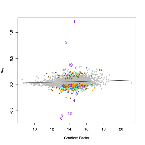
In this example, samples are colored by lab / chiptype: Red -- site A, HG-U95A; yellow -- site A, HG-U95Av2; black -- site B, HG-U95A; gray -- site B, HG-U95Av2; cyan -- site C, HG-U95Av2. Males are plotted as triangles, and females are plotted as circles (see PC Plots). Genes are colored as follows: Green -- negative controls; pink -- on X chromosome; blue -- on Y chromosome; purple -- on X and Y chromosomes; gray -- everything else. Moreover, genes from the Y chromosome are plotted as using their gene name, instead of the standard circle symbol.
The file my_ruv_plots_and_tables.R contains all of the plot routines in the ruv.extras package, but the names of the routines have been given the prefix "my_". For example, "ruv_scree" is renamed "my_ruv_scree." Therefore, you can easily edit the routines in any way you wish, source the file, and then use your version of the plot routines simply by adding the prefix "my_" in any of the code that calls the routines.
The file my_ruv.R is similar in nature. This file contains the script my_ruv_starter_analysis (and supporting subscripts). The only difference is the prefix "my." Thus, if you source the files my_ruv_plots_and_tables.R and my_ruv.R you will have all of the functionality of the ruv.extras package, just all the routines now have a "my" prefix. Of course, now you can edit these files however you like.
my_ruv.R is a rather complicated file, especially when you first look at it. Thus, before tackling this file, it is recommended that you first examine the file my_ruv_simplest.R. This script also contains a version of my_ruv_starter_analysis, but it is greatly simplified. This version does not create a web page. Instead, it simply outputs text and plots to the screen. Also, some of the less important options have been omitted. This script is great for understanding what my_ruv_starter_analysis does. It is also a great script to edit when you wish to create your own analysis.
Finally, my_ruv_simpler.R is somewhere in between. This version does not create a web page, but it does at least save the plots to disk. Once you have an understanding of my_ruv_simplest.R you may wish to examine this file, either as a next step in understanding my_ruv.R, or simply as a convenient way to save any plots you create to disk.