Contents

1 Introduction

The long-lived neutral Kaon K_L has rare decay K_L → π⁰νν which is a CP violating process. It happens at very low rate, and the branching ratio for this process to happen is calculated to be (2.49 ± 0.39 ± 0.06) × 10^-11[?] with very small theoretical uncertainties. It has attracted particle physicists’ interests in its ability to test the Standard Model (SM) by giving accurate measurement of Cabibbo-Kobayashi-Maskawa (CKM) matrix element parameters. Also, as a flavor changing neutral current (FCNC) process, the mechanism behind this process is forbidden at tree level in the SM, and can only proceed through higher order diagrams. The rate is therefore very sensitive to short distance effect, i.e. high energy scale effects beyond the current accelerator energy scale. As a result, it is an excellent tool for probing the Beyond Standard Model (BSM) extensions which are at energy scale at TeV.
In this chapter, we will start with the brief description of Kaon phenomenology by giving the basic terminology, focusing on its CP violating properties. Following that will be the discussion on how the branching ratio measurement of K_L → π⁰νν will be a good tool to test the SM. It will be followed by the prediction of the branching ratio from different BSM extensions.

2 Kaon Phenomenology

The most astonishing phenomenon in K meson system is CP violation. There’re three important discrete symmetries in quantum field theory: Charge conjugation (C), i.e. convert the particle to its anti-particle; parity (P), by inverting the spatial coordinates and time reversal (T), meaning time inversion. CP violation means that theory (electroweak theory, specifically) is not invariant under the combinational action of charge conjugation and parity. For example, the long-lived Kaon K_L is mostly a CP odd state, i.e. CP = -. And also, a neutral pion π⁰ has parity eigenvalue -1, since it’s a pseudoscalar. A state of two π⁰s, if the total momentum L is 0, has paritiy equals (-1)^2+L = 1. If CP is conserved, the K_L cannot decay ino π⁰π⁰ state via weak interaction. But experimentally, people observed this to happen but at very low rate. Moreover, field theory assumes CPT to be a good symmetry. So for CP violation processes, the T inversion will not hold any more.

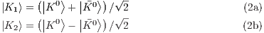
The K mesons, and its charge conjugation form strong isospin = 1∕2 doublets. For the neutral Kaon system, the two strong eigenstates K⁰ and K⁰ have quark constituents (ds) and (ds) respectively. In the context of the CP violation in the neutral Kaon system, neither K⁰ nor K⁰ are weak eigenstates. Instead, they follow the following equations

As a result, the CP eigenstates noted as K₁ and K₂ can be constructed via

Consequently, K₁ and K₂ will have CP eigenvalues -1 and +1, respectively. Life would be boring if the real life stable particles K_L and K_S (which stand for long-lived Kaon and short-lived Kaon), which are mass eigenstates such that they don’t oscillate, are the K₁ and K₂ with specific CP. In contrast, what happens is that experimentalist in the 60s detected decay K_L → π⁺π^-, and similar to the example given in the beginning of the section, this process is CP violating. There are two sources of the CP violation: indirect CP and direct CP violation. In the indirect CP violation case, the mass eigenstates K_L and K_S are not exactly the CP eigenstates, but with a little mixing coefficient ϵ:

The absolute value of ϵ is 2.3 × 10^-3. On the other hand, the direct CP comes from the weak interaction itself, and this effect is even smaller (denoted as ϵ^′). Experimentally, the real part of ϵ^′∕ϵ ≈ 1.67 × 10^-3.

3 K_L → π⁰νν in the Standard Model

3.1 The ”golden” Flavor Changing Neutral Current process

The flavor structure in the SM implies that in weak interactions, quarks with different flavors, i.e. from different families, cannot convert to each other without a change of charge. Such kind of processes is called Flavor Changing Neutral Current (FCNC) processes, where the neutral current is specific to Z₀ boson. A good example of FCNC vertex is s → dZ⁰, and this vertex describes processes like K⁰ → l⁺l^-, where l can be e,μ, or τ; K⁺ → π⁺νν, and most of all, K⁰ → π⁰νν.

Because such FCNC processes are forbidden at tree level in the SM, they can only proceed through higher order loop diagrams with two W^± interchanges which allows both the change of flavor and a conservation of charge. It’s known that loop diagrams are suppressed by the small weak coupling constant, and thus such FCNC processes are generally rare processes happening at very low rate. If there is a new theory, which provides new diagrams to the rare process and the rate is altered, then such deviation will be sensitively detected.
The energy scale these rare processes correspond to can be 100 TeV or higher, which provides a detour to measure high energy physics without building an expensive accelerator with higher beam energy. On the down side, FCNC processes are rare, therefore they usually require a high luminosity beam, and a good handle of the vast background.
To conclude, the FCNC process physics, usually called accurate measurement, is to measure rates or other quantities of SM highly suppressed processes. If any deviation from the SM is observed, it will be able to eliminate new physics or some parameter space of some new theories.

3.2 SM prediction of the branching ratio

The effective Hamiltonian describing K⁺ → π⁺νν and K_L → π⁰νν has the form [?]:

(4)

Different terms will be explained below: V _ij are CKM matrix elements which we will discuss in section 3.2.1, the first X_NL term describes the contribution from charm quark contribution, and the second term is where the penguine diagram contribution lies in with x_t = m_t²∕M_W², and X(x_t) is a monotonically increasing function with respect to x_t.

There are two types of diagrams contributing to the branching ratio shown in Fig. 1: the Z⁰ penguine diagrams and the box diagram. It is helpful to note that for the Z⁰ penguin diagrams, the internal top quark dominates due to its big mass, and the charm quark dominates the box diagrams because it has comparable masses compared to the leptons in the loop. The above Hamiltonian includes the next-leading-order and next-next-leading-order QCD corrections.

For K_L → π⁰νν, it has merits over K⁺ → π⁺νν. The reason is that the neutrino pair is in a CP even eigenstate, so this process is pure CP violating. As a result, the charm quark contribution is only approximately 1% , and can be neglected. So the branching ratio can be expressed as

(5)

where κ_L = (2.231 ± 0.013) × 10^-108.

Here, the λ is |V _cb| and the λ_t = V _ts^*V _td. K_L → π⁰νν has very small theoretical uncertainties. The K_L form factor does not depend on lattice QCD calculations, which has big uncertainties. Instead, it can be extracted from K_L semi-leptonic decay rates. The parametric uncertainties in the expression resides in three parts: m_t, Imλ_t and κ_L.
This section will be concluded by citing the numerical results for equation 5. the SM calculation on the K_L → π⁰νν branching ratio including 2-loop QCD and electroweak contribution is (2.43 ± 0.39 ± 0.06) × 10^-11, and total theoretical uncertainties is 2.5%. The first error is parametric uncertainties and the second error is from remaining theoretical uncertainties [?].

3.2.1 Accurate Measurement of the CKM Unitarity Triangle

The CKM matrix represents the transformation between the flavor eigenstates and mass eigenstates of three generations of quarks. V _CKM=

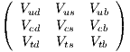
One property of the CKM matrix is that it’s ”mostly diagonal”. Numerically, the off-diagonal entries |V _us| = 0.23, and |V _ub| = 4.2 × 10^-3. To better show the mostly diagonal structure of the CKM matrix, people uses the Wolfenstein parameterization defined below.

The equation 6c looks very cumbersome and unnatural, but it turns out that with this definition, the parameters ρ and η will be the apex of the Unitarity Triangle (UT), which will be discussed further.
CKM matrix is a unitarity matrix, i.e.

(7)

This equation, if drawn in the complex plane, will form a triangle for which the vertices are (0,0),(1,0) and (ρ,η). The equation 5, if represented in the wolfenstein parameters, will become

(8)

So the branching ratio of K_L → π⁰νν is proportional to the height of the unitarity triangle. Accurate measurement of K_L → π⁰νν branching ratio therefore can give accurate measurement of CKM parameter η in lack of hadronic uncertainties.

We will not dig into the similar discussion for K⁺ decay but will simply cite the result: the branching ratio of K⁺ decay is proportional to one side of the UT as shown in Fig. 2. There exists a ’golden relation from which the measurement of the two branching ratios can determine the UT completely. Specifically, the angle β can be measured with high accuracy free from any hadronic uncertainties. At the same time ,the angle β can also be derived from another path of the CP asymmetry of B → ψK_S decay. When considering the BSM extensions, however, the golden relation will be broken in different ways and can be experimentally identified.

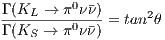
3.3 Grossman-Nir bound

We’ve seen that it is hard to talk about K_L → π⁰νν without constantly referring to its charged counterpart K⁺ → π⁺νν since they both go under the same Feynman diagrams at quark level. There’s a bound called Grossman-Nir bound which gives an upper limit on the branching ratio of the neutral decay with respect to the charged decay by giving[?]

(9)

The bound is derived from only the isospin symmetry and is model independent. The angle θ is defined to b rhe relative phase between the K -K mixing and s → dνν decay amplitude. And the following identity is straightforward to be derived:

(10)

At the same time, isospin symmetry gives A(K⁰ → π⁰νν)∕A(K⁺ → π⁺νν) = 1∕. Considering the isospin breaking factor to be 0.954[?], and the lifetime of the two Kaons τ_KL∕τ_K⁺ = 4.17, the equation 9 can be obtained.

4 Probing the Beyond Standard Models

We’ve known that the complex phases in the off-diagonal elements of the CKM matrix will contribute to the CP violation. Then the question to ask is whether such contribution is enough. The Hamiltonian describing the Kaon decays in equation 4 is generic and model independent. For various beyond standard Models (BSMs), the difference entirely resides in the funtion X(x_t) and an additional complex phase is brought in.

(11)

In the next few sections, the impact of different BSMs on the amplitude or the complex phase of the X function will be reviewed.

4.1 BSMs with Minimum Flavor Violation (MFV)

MFV is a catagory of simplest SM extensions. Under MFV assumption, the contribution of new operators not present in SM is neglegible, so only the (V-A) ⊗(V-A) operators identical to equation 4 are kept. And the phases in the CKM matrix is still the only contribution to the CP violation. All the SM extensions with MFV have the complex phase θ_x = 0 or π. However, they affect the amplitude by introducing diagrams with new particles in the internal loop.
To be explicit, the function X(x_t) should be replaced by a real-valued function X(ν) and ν represents a set of parameters of a given MFV model. Moreover, the X(ν) function can be either positive or negative according to different θ_x (Later analysis shows that the negative solution is neglegible). The model independent result which is related to K_L → π⁰νν is that it gives a tighter bound of its branching ratio with respect to K⁺ → π⁺νν shown below:

(12)

where B₁ and B₂ are the reduced branching ratios: Br(K⁺ → π⁺νν)∕κ⁺ and Br(K_L → π⁰νν)∕κ₀ respectively, and the angle β is unfixed but can be calculated from a_ψKs, and σ is a constant equals ². Recall the latest experimental result of K⁺ → π⁺νν branching ratio measurement: (Note: this result is 2004 result, need to update the results with 2008 result) [?]

(13)

and a_ψKS ≤ 0.719, we can get in MFV models, the upper limit of K_L → π⁰νν branching ratio is 2.0 × 10^-10.
To conclude, with the improved measurements of a_ψKs from B meson decays, the MFV extensions will not allow too much deviation from the SM. This indicates that if large deviation of the branching ratio is observed (a factor of 2 larger, for example), new CP violating phases must exist.

4.2 SM extensions with large θ_X

We start with a model independent discussion. In this case, the X(x_t) function will be complex as expressed in equation 11. The K_L branching ratio is changed to

(14)

where β_X = β - β_s - θ_X, and β and β_s are phases of V _td and V _ts. Figure 3 shows the branching ratios of K⁺ and K_L decays with scanning different values of β_X and |X|.

4.2.1 Littlest Higgs Model with T-parity

The Littlest Higgs Model is that the global SU(5) symmetry is spontaneously broken into SO(5) at 1 TeV energy scale, and new particles are introduced including the heavy gauge bosons W_H^±, Z_H and A_H, the heavy top T and scalar triplet Φ. One of the merits of the Littlest Higgs models is that it resolves the quadratic divergence of the Higgs mass by introducing new diagrams from these new particles. One of the series of Littlest Higgs Model that is very sensitive to K_L → π⁰νν branching ratio is the Littlest Higgs model with T symmetry(LHT). With this extra symmetry requirement, new quarks and leptons are introduced. Their interactions with the SM quarks involves new unitarity matrices, and new flavor violating phases are introduced therein. Here, we simply cite the relevant result without digging deeper into theoretical discussions. First of all, a large range of |X| and θ_X can be predicted:

(15)

As a consequence, an enhancement of the K_L → π⁰νν branching ratio is possible. Fig. 4 shows the predictions of the two Kaon branching ratios under different senarios of LHT, as shown by different colors. We can observe two branches, one of which shows no significant deviation from the SM, where the other shows large enhancement of the neutral mode, assuming that the K⁺ branching ratio is less than 2 × 10^-10.

4.2.2 Minimal Supersymmetrical Model

Minimal Supersymmetrical Model (MSSM) is another way to resolve the Higgs quadratic divergence by doubling the number of fields. Flavor violation is natural from the Yukawa superpotential. In the superpotential, relavant terms are expressed

(16)

[?] where λ_u^ij and λ_d^ij are the coupling constants between family i and j, which is similar to the CKM matrix. Q, U and D are chiral multiplets, and H_u and H_d are two Higgs fields. In general, the two coupling matrices cannot be diagonalized simultaneously, so terms violating flavor number exist. One of the mechanisms is to introducing diagrams from chargino loops and neutralino loops shown in figure 5[?]. The other of the mechanisms for enhancement is from charged Higgs mediated penguine diagrams in the region of large tanβ whose diagrams are shown in fig 6[?]. In both cases, sizable deviation from SM is possible within some parameter range.

4.2.3 Z^′ models

Z^′ is proposed in different BSMs and is able to mediate FCNC at tree level. [?] From a general point, the mass of the Z^′ and the coupling constant (for example, how the left-handed current and right-hand current couple), will determine the branching ratios. As shown in figure 7, in different charge coupling senarios and different masses, sizable deviation can be expected, but with increasing Z^′ mass, the abundance is reduced.