Classical treatments of the problem are mostly based on the approximation of the surfaces as a set of `asperities' of idealized shape (e.g. ellipsoids). The real surfaces are represented as a statistical distribution of such asperities with height above some datum surface. The contact of a respresentative asperity is analyzed, based on a micromechanical contact model, and the ensemble effect of all the contacting asperities is then constructed by superposition.
The most widely used asperity model theory is that due to Greenwood and Williamson (1966). They showed that if the height distribution of asperities is exponential, the relationship between bulk quantities such as total actual contact area, total normal force, total electrical conductance and total frictional force is linear regardless of the assumed asperity shape or micromechanical deformation mechanism. Real asperity distributions are of course not exponential, but many approximate Gaussian distributions and for this case, Greenwood and Williamson showed that the deviation from linearity in these relations is extremely weak over many orders of magnitude. This arguably provides the most convincing explanation of Coulomb's law of friction - the theory that the limiting frictional force is linearly proportional to the normal force.
This feature of finer and finer detail becoming clear as the measurement length scale is reduced is characteristic of the mathematical objects known as `fractals'. Many authors have therefore proposed to replace the asperity model concept by a description of a surface as a fractal. The trouble is that there is no obvious way to solve the contact problem for two fractal surfaces, or for one fractal surface contacting a plane. The most widely accepted fractal theory is that due to Majumdar and Bhushan (1990) in which the distribution of contact areas is tied to the distribution of `islands' cut off from the surface by a given horizontal plane as shown in Figure 1. This is a classical quantity in fractal theory. Majumdar and Bhushan replace the material in each island by a smooth parabolic asperity, thus effectively defining a fractal distribution of asperities that can then be treated as in a conventional asperity model.
 If the points A,B in the profile are defined, the mid-point C is chosen to deviate from the linear interpolation point C' by a vertical distance chosen using a random variable scaled with a power of the horizontal length scale xB-xA. The scaling parameter determines the fractal dimension of the resulting surface.
Borri-Brunetto et al. then discretized the corresponding elastic contact problem using a rectangular mesh. Numerical results for finer and finer meshes are equivalent to the use of progressively reduced sampling length in the fractal description.
The fractal dimension of quantities such as the total contact area was then determined by plotting the numerical results as a function of mesh size. Contact areas at each scale resolved into clusters of smaller contacts at the next smaller scale, with a consequent reduction in total contact area. The fractal trends suggested that the final contact area would be an infinite set of point contacts of total measure zero. This is definitely inconsistent with fractal models based on the `island' cross section.
 He made the approximation that the total force would be shared by the resulting microcontacts in proportion with the contact pressure in the smooth case. This is broadly equivalent to the theory that highly clustered contacts act as a single contact equal to the envelope size (Greenwood 1966).
Archard used his model to show that the elastic Hertzian relation between force and total contact area becomes more and more linear as fine scale roughness is added.
The constant of proportionality also gets smaller as more scales are added and actually tends to zero in the fractal limit, but Archard didn't remark on this result. The same effect is observed in the Greenwood and Williamson model as more and more scales of microscopic asperities are added.
It is interesting to note that Archard's model is fractal, even though the terminology had not been invented at that time.
The results confirmed those of Borri-Brunetto et al. The total contact area is a fractal and tends to measure zero in the limit. Since the Weierstrass profile is not a true fractal (it has a largest scale --- the first sine wave in the series), the results are not exactly self-affine at the first few scales, but they approach this behaviour above a relatively small value of n.
A crucial question is `what happens to the relation between force, compliance and electrical contact resistance in the fractal limit? For an infinite set of point contacts, the total contact resistance might be anything between zero and infinity, since there are an infinite number of parallel paths through the contact, each of which has zero conductance! It seems plausible (based on Greenwood's cluster argument) that the electrical contact resistance would tend to a finite limit, but how might we find this limit?
Measurements of actual surfaces are necessarily `truncated' because of the finite dimensions of measuring instruments and sampling lengths. If we could produce a rigorous solution of the contact problem for a truncated rough surface, could we place bounds on the error resulting from the neglected fine scale roughness? If so, how far do we need to go in describing the fine scale roughness in order to get a good measure of electrical contact resistance?
We first establish an analogy between the mathematical descriptions of the electrical conduction problem and the elastic contact problem. The electrical potential is governed by Laplace's equation and the interfacial plane is an equipotential surface. The elastic problem can also be cast in terms of a harmonic potential function and the analogous problem is that in which the normal displacement in the contact region is uniform, whilst the normal traction is zero outside the contact region. These boundary conditions define the incremental contact problem - i.e. the response of the system to a small increment of normal load. It follows that there is a strict linear relation between the contact conductance (reciprocal of the resistance) and the incremental normal contact stiffness that depends only on the electrical and elastic properties of the contacting materials.
We then use the reciprocal theorem to bound the incremental stiffness of the elastic contact between the solutions of two smooth contact problems. Combination of these two results yields the required bounds.
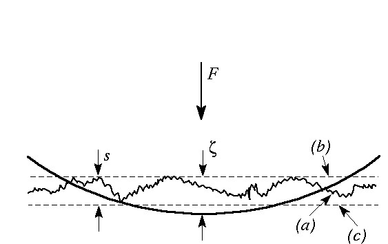 Suppose a rigid smooth indenter is pressed to a prescribed depth into
a half space with a rough surface, identified as (a) in the figure. We compare this state with two limiting smooth contact problems in which the rough half space is replaced by the smooth half-spaces (b) and (c) respectively. Surface (b) passes through the highest point of the surface and (c) through the lowest point, so that the real rough surface (a) is completely contained between (b) and (c). The vertical distance between these planes s is also the maximum peak-to-valley roughness of the surface Rt.
Suppose a rigid smooth indenter is pressed to a prescribed depth into
a half space with a rough surface, identified as (a) in the figure. We compare this state with two limiting smooth contact problems in which the rough half space is replaced by the smooth half-spaces (b) and (c) respectively. Surface (b) passes through the highest point of the surface and (c) through the lowest point, so that the real rough surface (a) is completely contained between (b) and (c). The vertical distance between these planes s is also the maximum peak-to-valley roughness of the surface Rt.
Common sense suggests that F(b)>F(a)>F(c) on the grounds that adding material to the half space above plane (c) can only make it harder to press in the indenter to the specified depth. The proof of this result is given by Barber (2003). However, notice that the roughness of surface (a) will generally cause the contact area A(a) not to be completely enclosed within A(b) or A(c).
The load-displacement relation for the smooth bounding surfaces (b) and (c) are similar but separated by a distance s. The curve for the rough surface A(a) must lie between these extremes.
It can be shown that the contact area A and the incremental stiffness must be non-decreasing functions of the indentation ζ, so the load displacement curve for both smooth and rough surfaces must be concave upwards. The limiting slope (incremental stiffness) at a given force F can therefore be bounded between two tangent lines. For more information on this procedure, please download the file Bounds on the electrical resistance between contacting elastic rough bodies.
In Figure 4, we show the bounding surfaces as planes because this simplifies the solution of the bounding contact problems, which then become Hertzian. However, the argument does not depend on the bounding surfaces being planes. For example, if we have a solution for the rough surface contact problem at some finite level of resolution, the effect of features below the resolution truncation can be assessed by defining two parallel surfaces separated by the maximum peak-to-valley variance of the scales neglected. The finite roughness problem might be solved by direct numerical methods such as finite element (Hyun et al. 2004), or by an asperity model theory with the asperities defined at some finite scale. This provides a means to tighten the bounds in practical cases. It also demonstrates that the 'infinite tail' (e.g. the terms beyond some fairly large number in a Weierstrass series) of a theoretical fractal distribution have negigible effect on the electrical resistance. Put another way, the resistance is largely determined by the coarse scale properties of the rough surface, which supports more recent arguments about asperity models due to Greenwood & Wu (2001).