Project Overview

Goals

This project aims to analyze the DSP used by the controller in an inverted pendulum system. To this end, our team has observed the effect that the gains, filter coefficient, and sampling rate of a PID controller has on the quality of control provided to the system (i.e. how long the pendulum is able to stay upright). Furthermore, we have found the LCCDE of the PID controller as well as its pole-zero plot with varying parameters to see how both change with respect to the level of control of the pendulum.

This Website

Below you will find a description of the model used in this project as well as a description of the PID controller used during simulation. On other pages of the website, you will see progress reports of our project to see how it developed over time as well as our final results of the project. On our Videos page, you will be able to see how the data generated by our model appear in a more physical form. You will be able to download the files we used in our project to play with the data on your own. Finally you will be able to meet each team member and see the contributions of each on the members page.

Inverted Pendulum Physical Model

The model for our project is based on the principles derived for a Simulink tutorial developed by the University of Michigan in conjunction with Carnegie Mellon University and the University of Detroit Mercy. The tutorial may be found by following this link.

Our system is modeled by a thin rod acting as a pendulum attached to a movable cart. This system has two degrees of freedom including the horizontal motion of the cart and the angular motion of the pendulum. The movement orientations are summarized in Fig. 1.

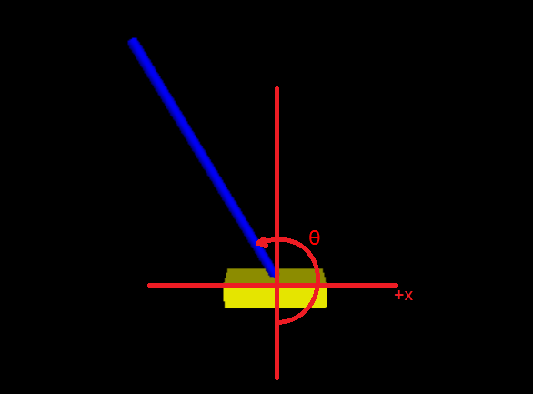
Fig. 1: Orientation of inverted pendulum

In the model, the pendulum rotates freely about its axis neglecting friction. The position of the cart is calculated by summing the external forces generated by the pendulum and PID controller, dividing by the mass of the cart to find its acceleration, and then integrating twice to find its position. The angle of the pendulum is found by finding the force exerted on the pendulum by the cart, dividing by the pendulum's moment of inertia to find its angular acceleration, and integrating twice to find its angle.

Fig. 2 shows the block diagram of our system which we created in Simulink. The physics of the inverted pendulum which were described in the previous paragraph are simulated in the "Inverted Pendulum System" block. The current position of the cart and angle of the pendulum as a function of time are generated as outputs to be read into the Matlab workspace and sampled by the "PID Controller" block.

The current angle of the pendulum is subtracted from its desired value (pi radians for vertical) before being sampled by the PID controller. From these samples, the controller calculates the proper force to apply to the cart to reduce the error and keep the pendulum upright.

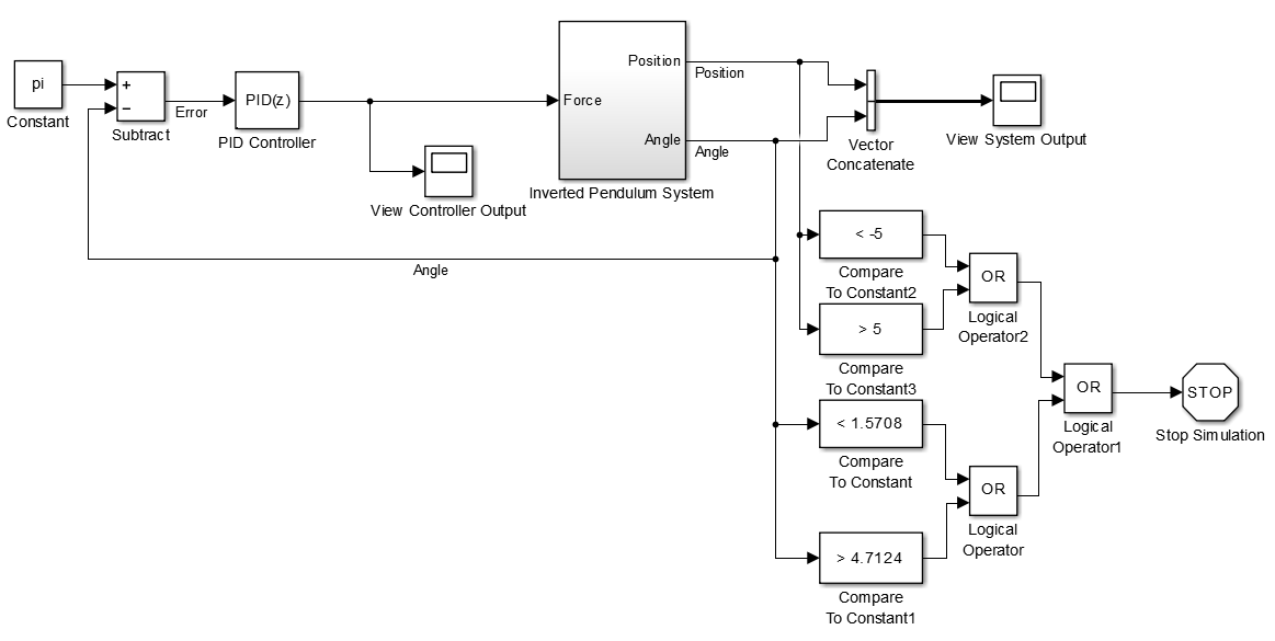
Fig. 2: The block diagram of the inverted pendulum control system created in Simulink

Furthermore, we applied a few physical constraints to the simulation. The simulation will be stopped and the controller will be considered to have failed if the cart moves more than 5 meters in either direction from its starting position. This will model the inverted pendulum system as having a limited track length in which it is able to move. In addition, the simulation will stop if the pendulum angle drops below horizontal to model the pendulum hitting the ground.

PID Controller

Our PID controller uses the following compensator formula. In the equation, P is the proportional gain of the controller, I is the integral gain, D is the derivative gain, N is the filter coefficient, and Ts is the discrete time sampling period.

Fig. 3: The Z-transform of the PID controller compensator formula

Matlab GUI

As part of our final project, we decided to make a GUI that a user can use to easily change the parameters of the simulation and see how the control of the pendulum is altered. Fig. 4 shows what the GUI looks like after it is opened and the "Run" button is pressed using the initial values.

The cart's position for the duration of the simulation is shown in red in the top right graph. The pendulum's angle is shown in blue in the second graph to the right. Seven sliders at the bottom right of the GUI are used to change the controller parameters as well as the initial angle of the pendulum and length of the simulation. Although the maximum length of the simulation may be set manually, the graphs will only plot the simulation data until the inverted pendulum system fails. The pole-zero map located at the top left calculates the current poles and zeros of the controller's Z-transform using the gains, filter coefficient, and sampling period slider values. The poles and zeros are also listed below the plot for readability. The Linear Constant Coefficient Differential Equation is calculated by taking the inverse Z-transform of the controller compensator formula and is displayed at the bottom left of the GUI. By hitting the "Run" button, the Simulink model will run using the current slider values and update all plots and equations. The "Reset" button will change the slider values back to their original magnitudes.

Fig. 4: The Matlab GUI