3D Atlas of Ann Arbor:
The Google Earth® Approach

Part I

Sandra Lach Arlinghaus

Note:  Google Earth
® and Google SketchUp® are both names trademarked by Google®.


The virtual reality files in the first edition of the 3D Atlas of Ann Arbor were all made using a strategy involving Geographic Information System (GIS) software coupled with 3D graphic design software.  The process was effective but often time-consuming and the files created were quite large.  Indeed, in the latter vein, alternative strategies, such as linking one file to another in a hierarchical pattern were employed so that the reader never had too large a file on screen at a single time.  Another issue involving the creation of these files was cost of the software.  The process involved many thousands of dollars worth of software (and of time of experts using the software).  Small cities had faint hope of being able to maintain a state-of-the-art 3D system without substantial donations of time, software, or both.

Google Earth® offers a different approach.  The interactive Earth viewer is, by now, probably familiar to most readers of Solstice.  The spectacular shiny Earth-ball causes most to exclaim at its beauty on first sight.  Further probing of the interactive capability brings additional admiration for its capabilities.  Figure 1, below, shows an animated set of images from Google Earth®.  It begins with the Earth and then zooms in to scenes of Chicago,. 
Notice that only the flat aerial has texture; the building surfaces have no textures on them, although many of the buildings have been modeled to look like reality--that is, they are not mere rectangles extruded to boxes.  The reader wishing to get a good look at Chicago should download Google Earth® (a free download from google.com) and drive around interactively within the model.  Then, try looking at a city that is familiar and see what memories emerge.


Figure 1:  Chicago scenes.

Beyond using Google Earth®, one might also be motivated to wish to create files to upload to Google Earth®.  Look, for example, at Ann Arbor in Google Earth®.   There is only a low resolution aerial (Figure 2) giving the viewer almost no information.


Figure 2.  Default view of Ann Arbor in Google Earth®.


One nice feature of Google Earth® is that one can upload aerials directly to the viewer and reposition them in relation to the coordinates already present.  Figure 3 shows more detailed aerials of Ann Arbor uploaded to Google Earth® (after being aligned with the coordinate system in relation to the location of the Huron River in downtown Ann Arbor).  Simply click on the "Add" pulldown and navigate to the files to be uploaded and then reposition them or resize them as needed.  The uploaded aerials are available in the library of The University of Michigan; the City of Ann Arbor supplied them to the author.  The first image in Figure 3 illustrates how the alignment was made with respect to the river.  The second image shows the image from Figure 2 with aerials superimposed.


Figure 3.  A better view of part of Ann Arbor (top) and a closeup of central Ann Arbor.


As was the case with Chicago, the flat aerials give a good view of the buildings; however, if one tips the image on its side, no buildings are displayed (Figure 4).  Unlike the case with Chicago, the Ann Arbor aerials are shot only in black and white.


Figure 4.  Ann Arbor, aerial only, lateral view shows no extruded buildings.

     With the memory of the beautiful scenes of Chicago in mind, it is easy to ask if one might upload 3D images of Ann Arbor (or elsewhere) into Google Earth®.  Another free download from Google®, called "SketchUp®" does indeed permit such uploads.  The premise is elegant:  the aerials uploaded into Google Earth® are coordinatized by virtue of their proper placement in the Google Earth® coordinate system.  Google SketchUp® permits the direct download of these aerials while retaining the coordinate information.  In SketchUp®, the user can add 3D buildings (digitizing them from the aerial and subsequently extruding them), model the buildings, apply photographic textures to them, set shadows, and a host of other operations.  When done, simply press the upload button and the buildings will be uploaded back to Google Earth® in the correct position on the globe using the embedded coordinated system.  Information lost in the upload is building material textures; only the flat surface textures of the aerial transfer through the interface.  Perhaps future versions of the Google Earth/SketchUp® pair will permit such upload.  The sequence of images below, in Figure 5, shows some of the features of SketchUp®.


Figure 5.  Downtown Ann Arbor (part) displayed in Google SketchUp®.


     The files created from SketchUp® for upload into Google Earth® are quite small in size so that one can imagine creating a great many buildings and still having the files run smoothly.  Figure 6 shows the upload of the material in Figure 5 to Google Earth® (important:  turn off the terrain switch in Google Earth®).  While the photographic textures do not upload, their influence is present as the buildings are more than the uniform shade of light gray (as in the Chicago file).  Scale of buildings and other objects is made easy from photographs coupled with the onboard "tape measure" in Google SketchUp®.  One might model any level of detail for the buildings, for street furniture, and so forth.


Figure 6.  Google SketchUp® materials uploaded to Google Earth®.


     The modeling of buildings, as opposed to the mere extrusion of buildings from digitized footprints, is quite straightforward once one works through the interactive tutorials.  Another useful feature is the ability to set shadow patterns according to month of the year and time of day.  Figure 7 shows an animated sequence of two views of the downtown, emphasizing shadow position at noon in each of the 12 months.  The darkest shadow is that inherited from the aerial; watch the lighter gray shadow dance across it.  When the SketchUp® files are uploaded to Google Earth® (Figure 6), the shadows do not upload.  The shadow present in the Google Earth® image is that photographed in the uploaded aerial.


Figure 7.  Animations emphasizing shadow position.

    
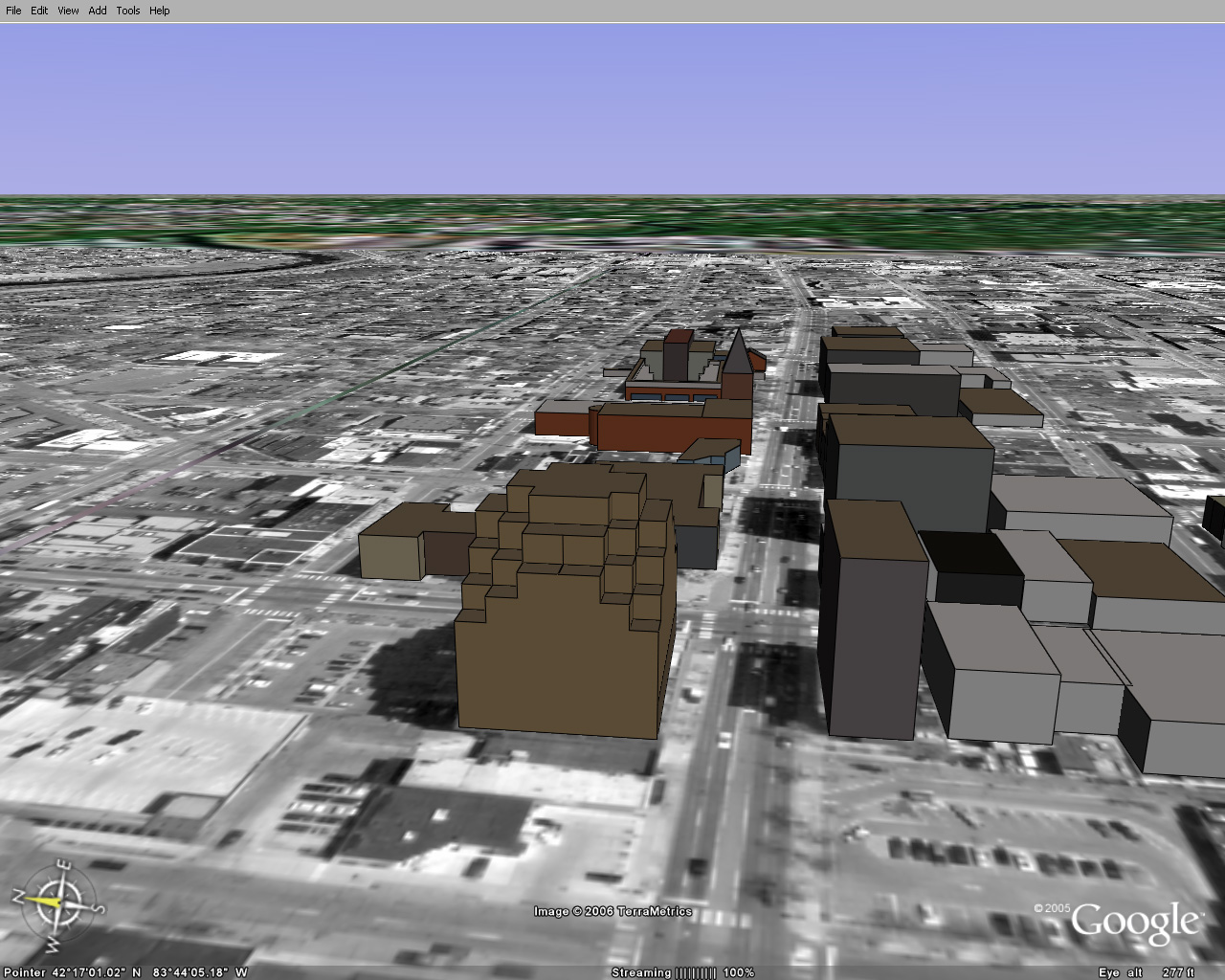
The images in Figures 1 to 8 are all based on screen captures from interactive products.  As such, they present only a small part of the story.  To see the Ann Arbor files, in Google Earth®, download Google Earth® to your hard drive.  Save the following files to your desktop (scanned by Norton and virus-free at upload):
Then, in Google Earth®, go to Open and navigate to the files on your desktop and open each of the three.  Then, type in "Ann Arbor" and you should be able to navigate the buildings for yourself!  Notice the compass.
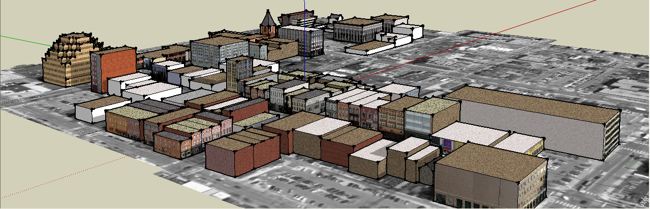
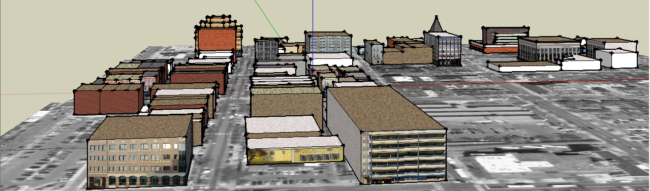
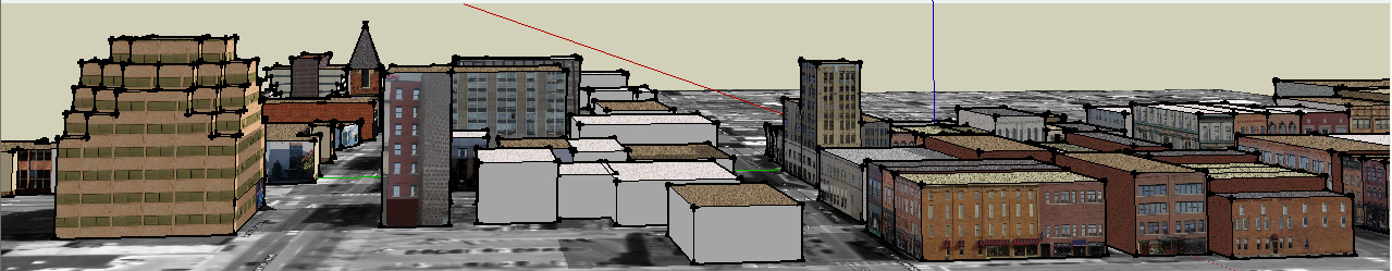
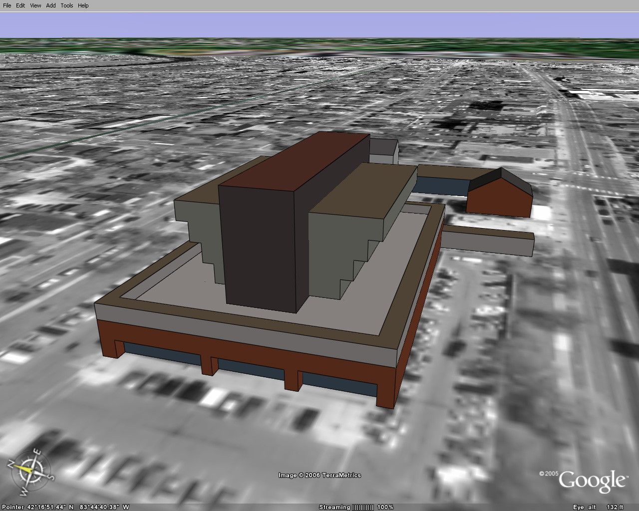
If you wish to view the scene with the photographic textures and shadows at varying positions, or to add new buildings of your own as an experiment in planning, then download Google SketchUp® (link below with the library of textures used) and install it and also download the SketchUp® file and Open it in SketchUp®.
  • SketchUp® executable file with suitable library:  Link 4.
  • SketchUp® file of Ann Arbor:  Link 5.
During the past 6 months presentations of the 3D Atlas of Ann Arbor, 1st Volume  (without Google Earth/SketchUp®), were given by the author to various groups of community leaders.  Particular wishes, beyond what was presented in that material were:
  • a desire to model buildings
  • a desire to introduce detail at the level of a single building (awnings, window displays, design elements of the building, and so forth)
  • a desire to measure the effect of shadows
  • a desire to be able to add buildings oneself, in considering possible sites for future buildings
  • a desire to build an Ann Arbor game
  • a desire to be able to own easy-to-use software and do all of the modeling on a home computer, or a city council computer, with no additional purchase of software.
The Google Earth/SketchUp® package enabled the entire wish list.  It is an important tool to add to the glittering array of software already employed by many urban and environmental planners.
What remains, beyond the obvious (but time-consuming) completion of all buildings and field-checking of heights and facades, is:
  • to integrate the effect of terrain
  • to learn to transform the files into a format that will play out in an immersion CAVE or other interesting 3D visualizations.


On June 9, 2006, the author presented the material in this article to an invited group at the 3D Laboratory of the Duderstadt Center at The University of Michigan:  John Nystuen, Gwen Nystuen, Fred Goodman, Ann Larimore, and Bart Burkhalter.  Click here for photos from the event:  photo 1; photo 2.

The author thanks Michael Batty, University College London for his encouragement in with respect to the Google Earth® upload.  She thanks Lars Schumann of the 3D Laboratory of The University of Michigan for pointing her to Google SketchUp®.  She thanks Professor Klaus-Peter Beier (The University of Michigan College of Engineering) and the staff of the 3D Laboratory, as well as Matthew Naud (Environmental Coordinator, City of Ann Arbor), for their continuing interest and encouragement in all aspects of this project over the past 4 years.  Merle Johnson of the City of Ann Arbor kindly supplied images of various sorts for this and for related projects.  For a full list of all individuals associated with this project, please see the online 3D Atlas of Ann Arbor also on the IMaGe website.

Solstice:  An Electronic Journal of Geography and Mathematics, Institute of Mathematical Geography, Ann Arbor, Michigan.
Volume XVII, Number 1.
http://www.InstituteOfMathematicalGeography.org/