|
|
|
|
|
|
|
![]()
![]()
![]()
Three dynamical cores of three different general circulation models have been used in order to compare the models' performance. Two of the models are global weather prediction models which have been developed at the German Weather Center (DWD, Offenbach, Germany). The model GME, that is based on an icosahedral grid, is the forthcoming forecast model of DWD. It will substitute the current operational spectral DWD model GM at the end of 1999. The third model involved in this comparison is the weather prediction model IFS, which runs operationally at the European Centre for Medium-Range Weather Forecasts (ECMWF, Reading, England). The table below gives an overview of the three models and lists their characteristic features.
|
|
|
|
|
|
|
|
|
|
max: 132 km |
|
(top at 10hPa) |
|
|
|
|
|
|
(top at 10hPa) |
|
|
|
|
|
|
(top at 10hPa) |
|
Three dynamical core runs at a high horizontal resolutions have been performed to compare the models' climate. All runs cover a time period of 1440 model days. 900 days of this time period have been used to compute the time-mean values which represent the general model circulation. In addition, the data are zonally averaged (over one latitude). This focusses the comparison on the meridional (north-south) oriented atmospheric patterns.
The following section shows selected model results. The time-mean zonal-mean zonal wind and temperature are representatives of the mean circulation whereas the Eddy heat flux, Eddy momentum flux and the Eddy kinetic energy indicate the co-variance terms that establish the global transport mechanisms. All figures are linked to underlying figures that are bigger in size and can be used to analyze the patterns more detailed.As it is demonstrated in the next section all three dynamical cores produce a similar model climate. This result is impressive because the models are based on different numerical approaches. It shows that the dynamically forced circulation develops nearly independent of the specific numerical formulation.
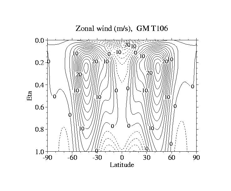
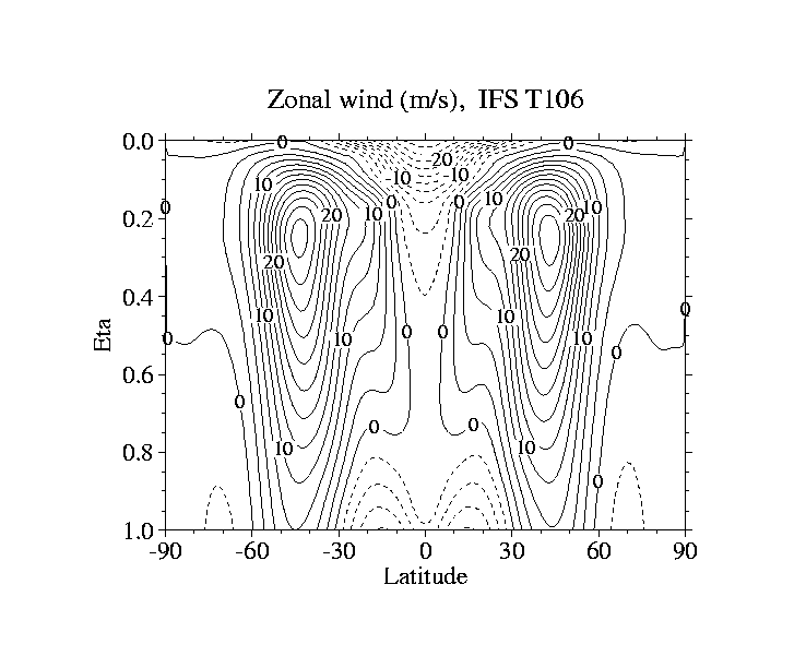
The figures below show the time-mean zonal-mean zonal wind patterns. The three models almost develop identical wind fields which especially becomes apparent when comparing the two DWD models GME and GM. Not only the strength and the shape of the jet streams are well-met but also their geographical positions. In addition, the comparison to the ECMWF model IFS reveals that the results nearly coincide. Small differences can only be analyzed in the upper atmosphere near the equator where the model IFS produces a slightly weaker band of easterlies. This phenomenon is possibly related to the semi-Lagrangian advection scheme whereas the two DWD models use an Eulerian approach.
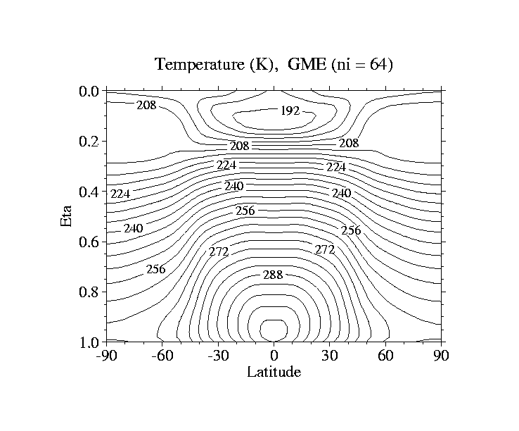
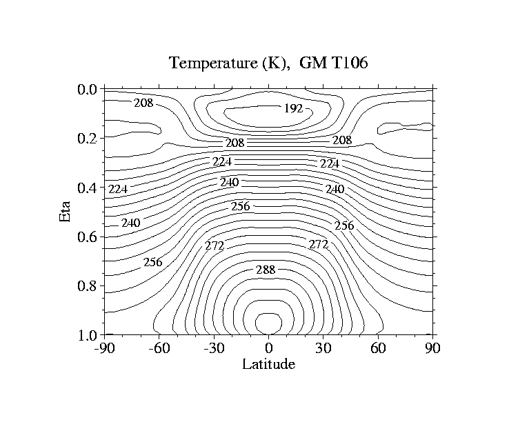
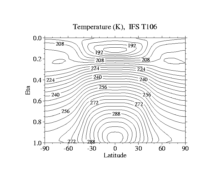
The time-mean zonal-mean temperature distribution of the three models is displayed below. These patterns show an idealized but typical temperature profile in the lower and middle atmosphere whereas the upper atmospheric regions (stratosphere and mesosphere) are unrealistically cool stratified. This is a consequence of the Held-Suarez forcing mechanism since it prescribes cool upper atmospheric temperatures that keep the stratosphere passive. The model comparison reveals that all three models produce a similar temperature pattern. Slight differences only appear in the upper atmospheric region near the equator. Especially the model IFS shows cooler temperatures at a height of eta=0.1 which approximately corresponds to a pressure level of 100hPa. Because of the close coupling of the temperature and zonal wind field (thermal wind relationship) this phenomenon might be related to the differences seen before when comparing the zonal wind pattern.
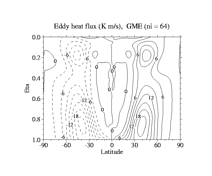
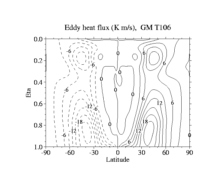
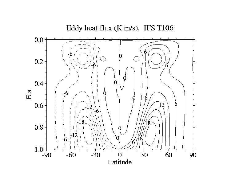
The Eddy heat flux shown below is a co-variance term that demonstrates an important energy (heat) transport mechanism. Heat gets transported from the equatorial regions to the poles by means of the atmospheric wave activity. This wave activity (low and high pressure systems) is concentrated on the midlatitudes. As a consequence, two transport maxima are located in the upper and lower atmospheric region in the midlatitudes. The model comparison demonstrates that all three models develop a similar transport pattern. Especially the flux maxima coincide with each other. This indicates that despite all numerical differences the three models are characterized by identical climatic features.
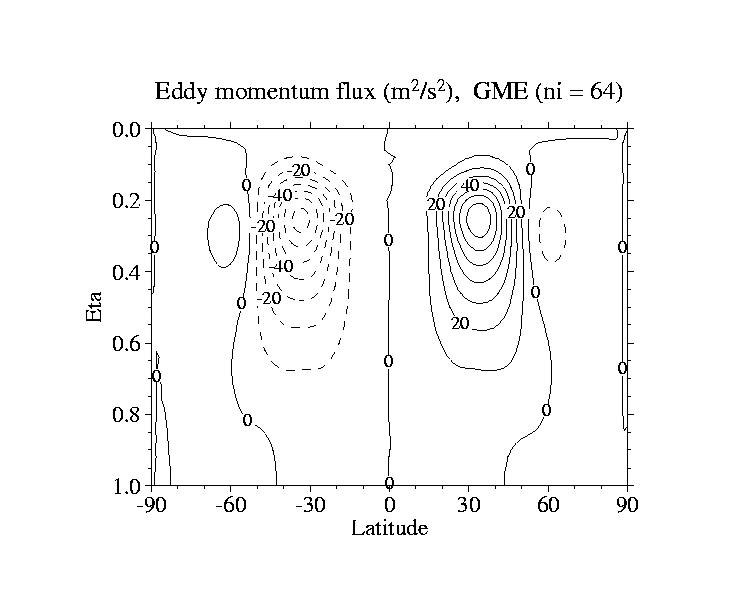
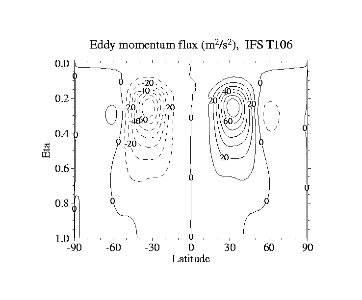
The Eddy momentum flux displays the transport of zonal momentum by the meridional (north-south) wind. This flux is important for the global circulation since it satisfies the global momentum balance equation. Zonal momentum gets transported from the equatorial region to the midlatitudes where a flux convergence zone can be found. This is as result of the global wind pattern which is characterized by easterlies in the equatorial region and westerlies in the midlatitudes. The zonal momentum is transferred by means of the atmospheric waves. In comparison to each other the models generate nearly coincident flux patterns. The maxima are located at the same geographical positions and their strengths just vary slightly.
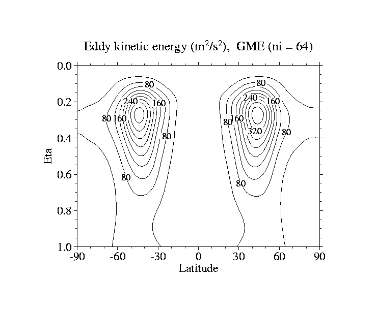
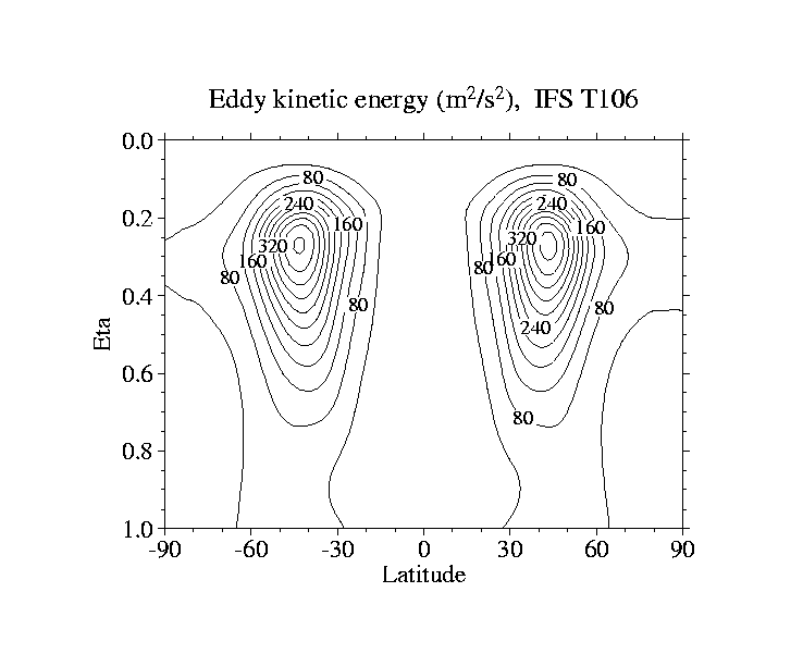
The figures below show the Eddy kinetic energy pattern of the three models. This co-variance term describes the strength of the wave activities in the models and therefore characterizes the meteorologically important low and high pressure systems. The wave activity is concentrated on the midlatitude regions. It becomes obvious that the location of the maxima approximately coincides with the position the zonal wind jet streams which have been displayed above. All three models produce a similar kinetic energy pattern with slight variations in the strengths of the fluxes. Especially the DWD model GME generates slightly less wave activity than the two spectral models GM and IFS. This could possibly be related to the different numerical approaches as the model GME is the only grid point model taking part in this comparison.
![]()
![]()
![]()