Torsten Hägerstrand, a Swedish geographer at the University of Lund, used the following technique to trace the diffusion of an innovation.

• The ‘thing’ being diffused (communicated) is an idea;
• the agents of diffusion, or carriers of new information, are human beings;
• the space in which the idea is to be diffused is a region of the world.

Hagerstrand traces the diffusion process by imitating it with numbers. Such imitation, leading to prediction or forecasting of the pattern of diffusion, is called a simulation of diffusion. To follow the mechanics of this strategy, it is necessary only to understand the concepts of ordering the non-negative integers and of partitioning these numbers into disjoint sets.

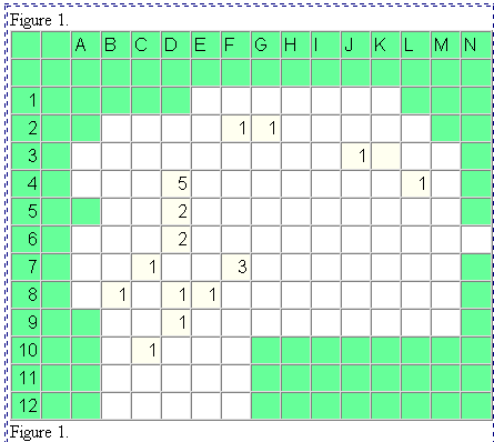
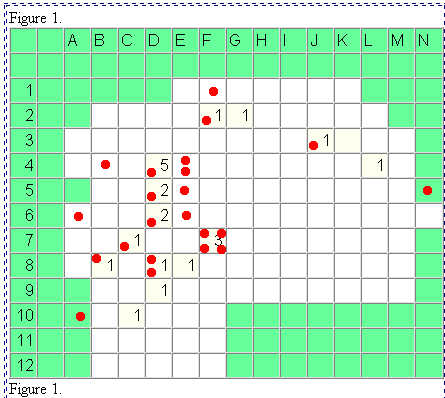
The figure on the left shows the spatial distribution of the number of individuals accepting a particular innovation after one year of observation (Hägerstrand, p. 380).  The figure on the right shows a map of the same region and of the pattern of acceptors after two years--based on actual evidence. Notice that the pattern at a later time shows both spatial expansion and spatial infill (more concentrated use and greater density per unit of land area). These two latter concepts are enduring ones that appear over and over again in spatial analysis---as well as in planning at municipal and other levels.
 

Might it have been possible to make an educated guess, from Figure 1 alone, as to how the news of the innovation would spread? Could the right-hand figure above have been generated/predicted from the left-hand figure using some replicable, systematic process? The steps below will use the grid in Figure 3 to assign random numbers to the grid in Figure 1, producing Figure 4 as a simulated distribution, as opposed to the actual distribution of Figure 2, of acceptors after two years.
 

• Construct a "floating" grid (Figure 3) to be placed over the grid on the map of Figure 1, with grid cells scaled suitably so that they match. Center the floating grid on a square in Figure 1 in which there exists an adopter (say 2F)...this is the first cell, working left to right and top to bottom, which contains a numeral. The numbers in the floating grid, used with a set of four digit random numbers, will be used to determine likely location of new adopters. It is assumed that the adopter in F2 (or in any other cell) is more likely to communicate with someone nearby than with someone far away (Tobler's Law--Newton...); velocity of diffusion is expressed in terms of probability of contact.

6248 0925 4997 9024 7754 7617 2854 2077 9262 2841 9904 9647 3432 3627 3467 3197 6620 0149 4436 0389 0703 2105

0000 to 0095 0096 to 0235 0236 to 0403 0404 to 0543 0544 to 0639 0640 to 0779 0780 to 1080 1081 to 1627 1628 to 1928 1929 to 2068 2069 to 2236 2237 to 2783 2784 to 7214 7215 to 7761 7762 to 7929 7930 to 8069 8070 to 8370 8371 to 8917 8918 to 9218 9219 to 9358 9359 to 9454 9455 to 9594 9595 to 9762 9763 to 9902 9903 to 9999

This assumption regarding distance and probability of contact is reflected in the assignment of numerals within the grid--there are the most four digit numbers in the central cell, and the fewest in the corners. The floating grid partitions the set of four digit numbers {0000, 0001, 0002, ..., 9998, 9999} into 25 mutually disjoint subsets.

FIGURE 4.  Here, the Mean Information Field collects new adoopters (red dots).  The transformation described above is animated to illustrate it.

Given a set (or sets) of four digit random numbers--as below. Center the floating grid on F2.  The first random number is 6248 and it lies in the center square of the overlay. So in the simulation, the acceptor in F2 finds another acceptor nearby in F2. Record that simulated acceptor as a red dot. Together with the original adopter, there are now two adopters in this cell.  Move the MIF over and repeat the procedure using the next random number in the sequence.

FIGURE 5.  Simulated distribution of acceptors, using random numbers.  Original acceptors in black; simulated acceptors in red.  Consider what to do with edge effect issues.  How does the simulation compare to the actual distribution of adopters after two years (Figure 2)?  This question leads to a whole set of issues about how to compare pattern--one might use color, contours, a variety of numerical measures, and so forth.  Attached is a rough idea using this particular small example.
 

a a A B C D E F G H I J K L M N  a a a a a a a a a a a a a a a a 1 a a a a a 1 a a a 2 a a 1+1 1 a a 3 a 1+1 a 4 a 1 5+1 1+1 1 a 5 a a 2+1 1 1 6 a 1 2+1 1 7 a 1+1 3+1+3 a 8 a 1+1 1+1+1 1 a 9 a a 1 a 10 a 1 1 a a a a a a a a 11 a a a a a a a a a a 12 a a a a a a a a a a

Construction of the floating grid--the so-called "Mean Information Field" (MIF) in the original example.

Assumption: the frequency of social contact (migration) per square kilometer falls off (decays) rapidly with distance.

The data are from an empirical study.

Units on axes: x-axis--distance in kilometers; y-axis--number of migrating households per square kilometer.

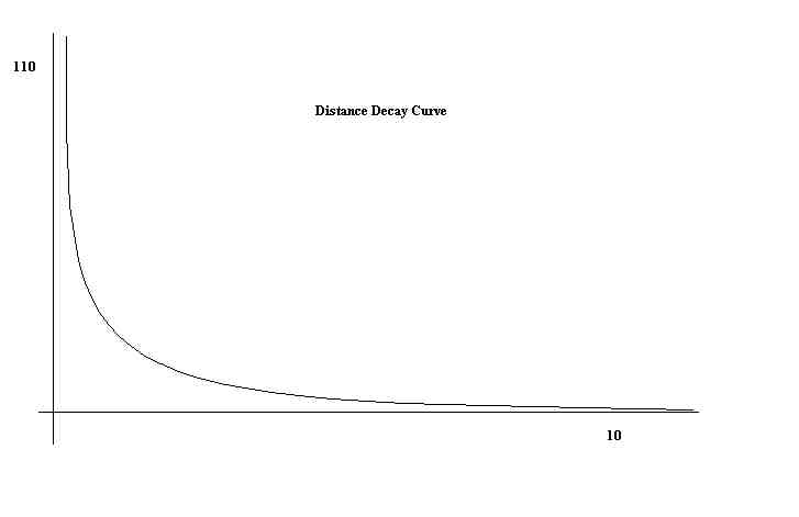
Definition:  An area containing probabilities of receiving information from the central point of that region is called a mean information field.

To assign quantitites of four digit numbers to each cell in the MIF, it is necessary to use the curve derived from the empirical study (distance decay curve).

It is used to

• determine the size of the MIF
• assign particular probabilities.

The size of the MIF is 25 by 25 kilometers squared. Observation is that the typical household moves no more than 12.5 kilometers. This field is then split into cells 5 by 5 kilometers squared.

Assignment of probabilities

From the graph of distance decay, a point 10 km from the center has a value of .167 associated with it. This is in households per square kilometer; there are 25 km squared in each cell; so the point value of the cell is 25*.0167=4.17. The center cell has a value of 110--an actual number of households.

The total point value of all cells is 248.24--note the symmetry caused by assumptions about ease of movement in all directions outward from the center.

Divide: 4.17/248.24=0.0168---so, assign 168 4 digit numbers to the cells that are 10 km from the center (two to the north, east, south, and west of center).

Thus, the Mean Information Field is constructed.

Some Basic Assumptions of the Simulation Method (Monte Carlo)

Assumptions to create an unbiased gaming table:

• the surface is uniform in terms of population and transport
• all contacts are equally easy in any direction
• there are an equal number of potential acceptors in each cell

• There is a set of carriers at the start (as in Figure 1)
• information is transmitted at constant intervals
• when carrier meets a new person, acceptance is immediate
• the likelihood of a carrier and another meeting depends on the distance between them.

Hägerstrand, Torsten. Innovation Diffusion as a Spatial Process. Translated by Allan Pred.  University of Chicago Press, 1967.