Research on Rates of Evolution
Introduction
Evolution is a process that takes place from one generation
to the next in living lineages of plants and animals. Evolutionary results are
sometimes visible on the time scale of
an individual generation, but we usually see and study these
cumulatively on longer experimental,
ecological/historical, and geological scales of time. Rates of
evolution are important because they
are a key indication of how the evolutionary process
works— rates quantify evolutionary change in relation
to time.
A process is a sequence of operations that produces a result.
Reading is a process. Readers read words, and the process can be described by
a simple rate, usually represented as words per minute. If a student reads 100 words per
minute, we expect that it will take him or her a
little over an hour and a half (100 minutes) to read a 10,000-word
book, and 16-17 hours (1000 minutes)
to read a 100,000-word book. The rate has to be
determined experimentally, of course, by counting the number of words read in a fixed amount
of time, or by measuring how long
it takes the student to read a text of some known length. Then a simple rate is calculated by
reducing the resulting quotient: e.g., 10,000 words per
100 minutes reduces to 100 words per minute, and the
result is assumed to be independent
of both the numerator and
denominator. This assumption of independence, rarely tested, is implicit in our everyday use
of simple rates.
The tricky part about a rate is that it is a ratio with a
numerator and a denominator (rate and ratio have
the same etymological root).
In the example here, the numerator is
words and the denominator minutes. When we reduce the
ratio we assume that readers read at the same
rate no matter how long the text. This could be true, but
even reading might be a little more complicated.
How long does it take a mouse lineage to evolve to double its size?
The answer depends, of course, on the rate— how fast is evolution?
Empirical observations
Rates of evolution are generally calculated in terms of proportional change,
ln (x2 / x1) = ln x2 − ln x1,
divided by elapsed time. The reasons for logging
measures of morphology are reviewed in
Gingerich (2000).
J. B. S. Haldane (1949) proposed a rate calculation in a unit called the darwin that
requires two quantities:
(1) the difference between means of two samples of natural-logged
measurements, d = y2 − y1;
(2) the time interval between the samples, I = t2 − t1, measured or estimated in millions of years.
The resulting rate in darwins is:
D = d / I
A rate in darwins is expressed in terms of factors of e (base of the natural
logarithms) per million years, neither of which are intuitive units: e and millions
of years are perfectly arbitrary in this context; the units do not appear in genetic models;
there is an erroneous suggestion, or even implication, that evolution takes place on million-year time
scales (see below); and rates in darwins cannot be compared for measurements that have different
or unknown dimensionality
(Gingerich, 1993).
It makes much more sense to follow a lesser known suggestion of Haldane and
calculate rates of evolution in terms of proportional change divided by elapsed
time, in a unit called the haldane (Gingerich, 1993).
This calculation requires three
quantities:
(1) the difference between means of two samples of natural-logged measurements,d = y2 − y1;
(2) the pooled standard deviation of the samples,sp = √(sp)2,
where (sp)2 =
[(n1−1) (s1)2 +
(n2−1) (s2)2 ] /
(n1 + n2 − 2), where
s1 and s2 are the standard
deviations of the samples of natural-logged measurements; and
(3) the time interval between the samples, I = t2 − t1,
counted or estimated in generations.
The resulting rate in haldanes is:
Hlog I = Z / I ,
where Z = d / sp
Here the result is expressed in terms of phenotypic standard deviations per generation,
and the subscripted log I is a reminder that the result is dependent on time scale
(rates of most interest are H0 where I = 1 generation and log I = 0).
Quantification in haldanes requires knowledge about phenotypic variability but
this is really necessary in any case in an evolutionary study because, as Haldane himself wrote,
variation is the raw material of evolution. Standard deviations are components of
selection intensity and response. A generational time scale, rather than millions
of years, is the time scale on which evolution takes place. And finally, rates in
haldanes are independent of the dimensions of the underlying measurements. These
are all advantages of haldane rate units over darwins.
Empirically, when rates of evolution are calculated on
different time scales, the rates decline
systematically the longer the time interval being studied
(Gingerich, 1983, 1993, 2001; Figure 1). This is
not an assertion– it is an empirical observation that
anyone willing to compile rates over a
range of time scales can easily demonstrate for himself or herself.
A simple evolutionary rate of measured change and time
does not produce a number independent of the
denominator.
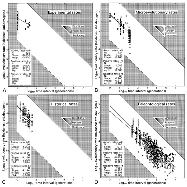
Figure 1.
Rates of evolution from different sources, calculated in haldanes on different scales
of time, and here scaled temporally against their denominators to make them comparable: (A) selection experiments
in laboratory and field; (B) 'microevolution'; (C) historical field study; (D) rates
from the fossil record. All predict rates on the order of 10-1 to 100
(0.1 to 1) standard deviations per generation on a time scale of one generation
(100; the time scale of the evolutionary process). Positive and
negative rates are distinguished to emphasize that these define upper and lower
bounds, respectively, of a distribution that is artificially hollow because very low
rates cannot be distinguished operationally from zero. Figure from Gingerich
(2001: fig. 8; sources of data are listed in original publication).
|
Reactions
Reactions to this
observation have been surprising. Paleontologists starting with
the late Stephen Jay Gould (1984) dismissed the observation of an inverse relationship of rates to their denominators as a
'psychological and mathematical artifact' of plotting a rate against its denominator.
Sheets and Mitchell (2001) call the dependence of rate on interval 'spurious self-correlation,' as if it somehow isn't real. Roopnarine (2003) calls the inverse relationship between rate and timescale a 'mathematical artifact predictable on the basis of the behavior of random walks.'
In response I reiterate, we calculate rates because we expect rates to be independent of their denominators, but independence is rarely what we see for evolutionary rates. There is nothing psychological or artifactual or spurious about plotting a ratio against its denominator to test their independence— and arguing that an inverse relationship of rates and intervals exists as an artifact is tantamount to arguing for independence when the opposite has just been demonstrated!
Rates are not independent of their denominators, and consequently they have to be evaluated in light of
the dependence, as was done, for example, by Mandelbrot (1967) in another
context— evaluating the length of the coastline of Britain.
Bookstein (1987)
interpreted the dependence of evolutionary rates on their denominators to
mean that evolutionary rates do not exist, just as, he argued, the length of
a coastline does not exist independent of its scale of measurement.
But existence dependent on scale is still existence. I agree that rates
of evolution are meaningless independent
of the time span over which they were calculated, but they
continue to have meaning as long as the time scale is known and specified.
Further, the natural focal time scale for evolutionary
studies— the generation-to-generation
or one-generation time scale— is the only time scale of interest
for evolution as a process. There is no shorter time scale, and results
on longer time scales (e.g., million-year time scales) are cumulative results reflecting evolutionary history but not the evolutionary process directly.
How Fast is Evolution?
Most of the rates of evolution that have been calculated and published over
the years, including those of Haldane (1949), were calculated based on fossil
lineages. Observed changes were very slow, and the rates were very low (indeed Haldane
had to invent the term "millidarwin" to express the rates he reported
for fossil lineages). Such emphasis on rates calculated from the fossil record misled all of us into thinking that evolution itself is
very slow.
What do rates of evolution in the fossil record tell us about evolution
on the generation-to-generation time scale of the process? Panel D in
Figure 1 answers this question: rates calculated from the fossil record are
very low: on the order of 10-7 to 10-3 haldanes or
standard deviations per generation. But when considered as they scale
relative to their denominators, rates calculated from the fossil
record project to rates of 10-1 to 100 standard
deviations per generation on a time scale of one generation. Such rates
are so high that they might
not be believable if they were not consistent with what we observe in the laboratory
and what we infer by scaling rates calculated on shorter time scales (panels A-C in Figure 1). For the
question— how fast is evolution in the face of selection?— the simple answer is 'fast' and the number to go with this is about one-tenth
of a standard deviation per generation. This is more or less an upper bound of course, but it
also expresses what we commonly see (Figure 1).
Accepting rates from the fossil record at face value— failing to
rescale to a timescale of one generation— explains several anomalous
results in the earlier literature. Lande (1976) inferred that
change in fossil lineages can be explained by as few
as one selective death per million individuals
per generation, and Lynch (1990) inferred that
rates of morphological change in fossil lineages are
substantially below the minimum neutral expectation. Both results are surprising, but
result from erroneously
assuming that rates calculated on
geological scales of time represent evolution on the
time scale of the evolutionary process (Gingerich, 2001). Natural selection operates statistically,
moment-to-moment, day-to-day, generation-to-generation, on the developing or mature phenotype (and hence
too on the underlying genotype) in front of it. The process has no memory nor anticipation. Selection
doesn't read a genetic code to act on some preceding or somefuture phenotype— it always acts
here and now. Hence the only rates of evolution that should be substituted in genetic
models like those of Lande and Lynch are generation-to-generation rates calculated on one-generation time scales.
A Rate Perspective on Punctuated Equilibria
and the Red Queen vs. Stasis Debate?
If the process of evolution is so dynamic on a generational scale of time, why does
it appear virtually stationary on longer scales of time? If you have read this far,
then you are ready for a thought experiment that helps to clarify both 'punctuated
equilibria' (Eldredge and Gould, 1972) and the debate over Red Queen evolution vs.
stasis? (Stenseth and Maynard Smith, 1984). The thought experiment is illustrated
in Figure 2, which is explained in the text on pp. 141-143 of Gingerich (2001).
Have fun!
Hint: Earth history and geological time have been orders-of-magnitude longer
than the evolutionarily-equivalent functional range of variation seen in even diverse groups of organisms. Morphology
is highly constrained relative to the time that has been available for evolutionary experimentation.
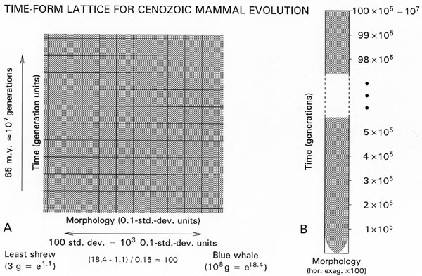
Figure 2.
Heuristic time-form lattice to explain
how evolution can be so dynamic in the short term, with H0 rates on the order of 0.1 standard
deviations per generation on the scale of one generation, and so static
over longer intervals. (A) If H0 rates are on the order of 0.1 standard
deviations per generation, then evolution takes place on a time-form lattice where a 0.1
standard deviation step or difference in morphology
corresponds roughly to a one-generation step or difference in evolutionary time.
The smallest living mammal is the least shrew weighing about
3 or e1.1 g, and the largest living mammal is the blue whale weighing about 100 metric
tonnes or e18.4 g. The standard deviation of body weight
in mammals is about 0.15 units on a natural logarithmic scale. Hence the largest and
smallest mammals living today differ by approximately
100 standard deviations or 103 0.1-standard-deviation units. These are physiological
limits and mammals have never been much smaller or
much larger: thus the time-form lattice for mammalian evolution is about 103 units wide.
The generation time for an average living mammal
is on the order of one year, and the Cenozoic history of the modern orders of mammals
as we know them goes back 5565 million years,
which is conservatively about 10 million or 107 generations. Thus the time-form lattice
for Cenozoic mammal evolution is about 107 units
long temporally. (B) The lattice is not square, but some four orders of magnitude longer
temporally than it is wide in form. Mammals starting
at some average size at the beginning of the Cenozoic can be expected to have diffused
and filled the lattice in less than 105 generations
[(500/1.96)2 65000 generations] less than one percent of their subsequent Cenozoic
history. Then they were constrained to evolve within
the lattice for the remaining 99 percent of their history. Rates of evolution on the
time scale of the process are so high that lineages rapidly find
and fill most niches within their physiological limits. Then they change little until
the system is perturbed. This, in other terms, is the evolutionary stasis model of Stenseth and Maynard Smith (1984). Figure from Gingerich (2001: fig. 9).
|
Gingerich Publications on Rates of Evolution (chronological order)
Gingerich, P. D. 1983. Rates of evolution: effects of time and temporal scaling. Science, 222: 159-161. Online or Request PDF/reprint 138
Gingerich, P. D. 1984. Punctuated equilibria-- where is the evidence? Systematic Zoology, 33: 335-338. Online or Request PDF/reprint 151
Gingerich, P. D. 1984. Smooth curve of evolutionary rate: a psychological and mathematical artifact-- reply to Gould. Science, 226: 994-996. Online or Request PDF/reprint 158
Gingerich, P. D. 1986. Temporal scaling of molecular evolution in primates and other mammals. Molecular Biology and Evolution, 3: 205-221. Online or Request PDF/reprint 173
Gingerich, P. D. 1987. Evolution and the fossil record: patterns, rates, and processes. Canadian Journal of Zoology, 65: 1053-1060. PDF or Request PDF/reprint 185
Gingerich, P. D. 1991. Fossils and evolution. In S. Osawa and T. Honjo (eds.), Evolution of Life: Fossils, Molecules, and Culture, Springer-Verlag, Tokyo, pp. 3-20. PDF or Request PDF/reprint 224
Gingerich, P. D. 1993. Quantification and comparison of evolutionary rates. In P. Dodson and P. D. Gingerich (eds.), Functional morphology and evolution, American Journal of Science, 293A (Ostrom volume): 453-478. PDF or Request PDF/reprint 258
Gingerich, P. D. 1993. Rates of evolution in Plio-Pleistocene mammals: six case studies. In R. A. Martin and A. D. Barnosky (eds.), Morphological Change in Quaternary Mammals of North America, Cambridge University Press, Cambridge, pp. 84-106. PDF or Request PDF/reprint 265
Clyde, W. C. and P. D. Gingerich. 1994. Rates of evolution in the dentition of early Eocene Cantius: comparison of size and shape. Paleobiology, 20: 506-522. Online or Request PDF/reprint 285
Gingerich, P. D. and G. F. Gunnell. 1995. Rates of evolution in Paleocene-Eocene mammals of the Clarks Fork Basin, Wyoming, and a comparison with Neogene Siwalik lineages of Pakistan. Palaeogeography, Palaeoclimatology, Palaeoecology, 115: 226-247. Online or Request PDF/reprint 291
Gingerich, P. D. 1996. Rates of evolution in divergent species lineages as a test of character displacement in the fossil record: tooth size in Paleocene Plesiadapis (Mammalia, Proprimates). In M. Godinot and P. D. Gingerich (eds.), Paléobiologie et Evolution des Mammifères Paléogènes: Volume Jubilaire en Hommage à Donald E. Russell, Palaeovertebrata, Montpellier, 25: pp. 193-204. PDF or Request PDF/reprint 316
Gingerich, P. D. 2000. Arithmetic or geometric normality of biological variation: an empirical test of theory. Journal of Theoretical Biology, 204: 201-221. Online or Request PDF/reprint 357
Gingerich, P. D. 2001. Rates of evolution on the time scale of the evolutionary process. In A. P. Hendry and M. T. Kinnison (eds.), Contemporary Microevolution: Rate, Pattern, and Process, Kluwer Academic Publishers, Dordrecht, Genetica, 112/113: 127-144. PDF (Deep Blue) or Request PDF/reprint 383
Gingerich, P. D. 2003. Mammalian responses to climate change at the Paleocene-Eocene boundary: Polecat Bench record in the northern Bighorn Basin, Wyoming. In S. L. Wing, P. D. Gingerich, B. Schmitz, and E. Thomas (eds.), Causes and consequences of globally warm climates in the early Paleogene, Geological Society of America, Special Papers, 369: 463-478. PDF or Request PDF/reprint 402
Gingerich, P. D. 2003. Land-to-sea transition of early whales: evolution of Eocene Archaeoceti (Cetacea) in relation to skeletal proportions and locomotion of living semiaquatic mammals. Paleobiology, 29: 429-454. Online or Request PDF/reprint 405
Gingerich, P. D. 2006. Environment and evolution through the Paleocene-Eocene thermal maximum. Trends in Ecology and Evolution, 21: 246-253. Online or Request PDF/reprint 441
Wood, A. R., M. L. Zelditch, A. N. Rountrey, T. P. Eiting, H. D. Sheets, and P. D. Gingerich. 2007. Multivariate stasis in the dental morphology of the Paleocene-Eocene condylarth Ectocion. Paleobiology, 33: 248-260. Online or Request PDF/reprint 458
Gingerich, P. D. 2007. Punctuated equilibrium (book review). Paleontologia Electronica, 10: 1-2. Online or Request PDF/reprint 469
Gingerich, P. D. 2009. Rates of evolution. Annual Review of Ecology, Evolution, and Systematics, 40: 657-675. Online/PDF or Request PDF/reprint 498
Other Publications
Bookstein, F. L. 1987 . Random walk and the existence of evolutionary rates. Paleobiology, 13: 446-464.
Eldredge, N. and S. J. Gould. 1972. Punctuated equilibria: an alternative to phyletic gradualism. In T. J. M. Schopf (ed.), Models in Paleobiology, Freeman, Cooper and Company, San Francisco, pp. 82-115.
Gould, S. J. 1984. Smooth curve of evolutionary rate: a psychological and mathematical artifact. Science, 226: 994-995.
Haldane, J. B. S. 1949. Suggestions as to quantitative measurement of rates of evolution. Evolution, 3: 51-56.
Koch, P. L. 1986. Clinal geographic variation in mammals: implications for the study of chronoclines. Paleobiology, 12: 269-281. JSTOR
Lande, R. 1976. Natural selection and random genetic drift in phenotypic evolution. Evolution, 30: 314-334.
Lynch, M. 1990. The rate of morphological evolution in mammals from the standpoint of the neutral expectation. American Naturalist, 136: 727-741.
Mandelbrot, B. B. 1967. How long is the coast of Britain? Statistical self-similarity and fractional dimension. Science, 156: 636-638.
Roopnarine, P. D. 2003. Analysis of rates of evolution. Annual Review of Ecology and Systematics, 34: 605-632.
Sheets, H. D. and C. E. Mitchell. 2001. Uncorrelated change produces the apparent dependence of evoutionary rate on interval. Paleobiology, 27: 429-445.
Stenseth, N. C. and J. M. Smith. 1984. Coevolution in ecosystems: Red Queen evolution or stasis? Evolution, 38: 870-880.
Page updated
1/28/10
: Comment?